Day 9: DCGAN and CVAE on CIFAR10

The previous post, I trained the model on a grayscale image, today I will train the model on a color image from CIFAR10 and STL datasets. It is much more difficult to make it work.

DCGAN

I just simply changed the model to take a color image by changing the number of input channels to 3 but got no luck. The model fails gracefully because the generator fools the discriminator with a garbage:

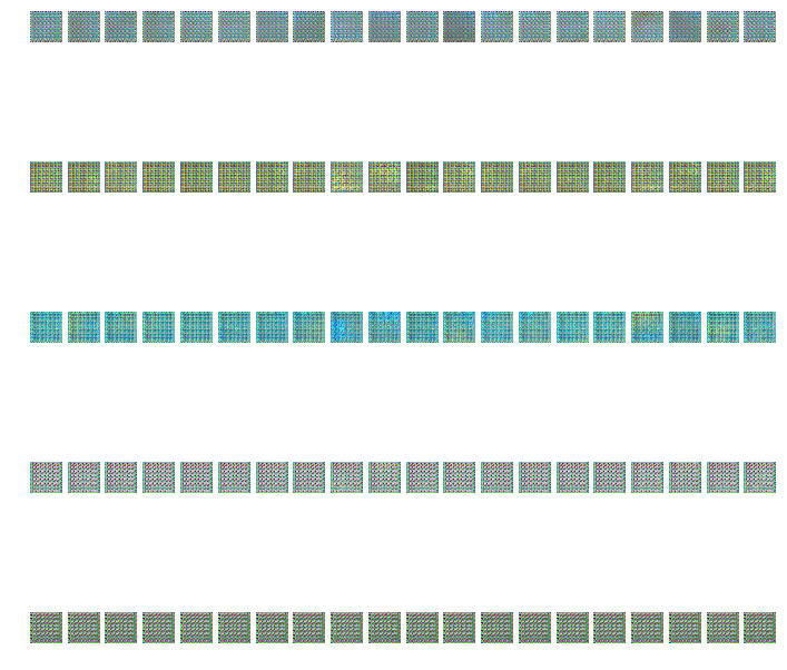
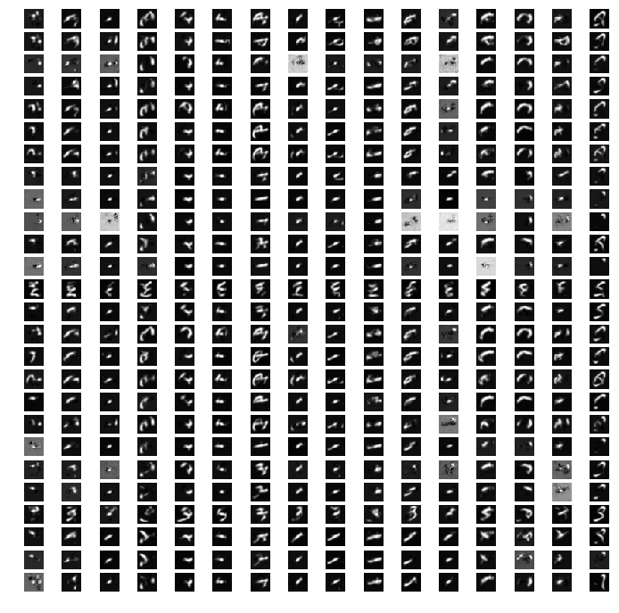
20 CIFAR images generated by the generator of DCGAN. The model cannot learn anything. Each row is the number of epochs starting from 10 (top), 50, 100, 150, and 200. Each column is a unique random vector sampled from a uniform distribution and used as the initial input to the generator.

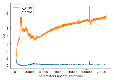
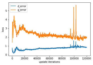
When we look at the loss, the generator performs better because the discriminator can’t distinguish anything.

After many trial-and-error, one change that works is to scale an image to 64 by 64 and normalize each color channel to have a center of 0.5 with a standard deviation of 0.5. I also use torchvision to plot an image which is very convenient than using matplotlib.

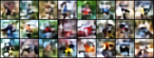
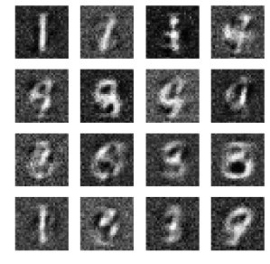
Here are generated CIFAR10 images from DCGAN:

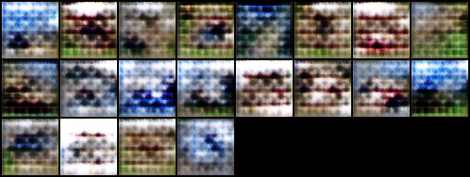
The generated CIFAR10 images after 10 epochs

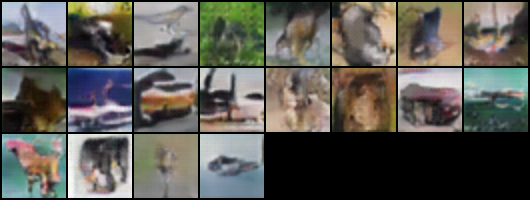
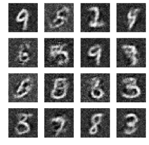
The generated CIFAR10 Images from the Generator after 150 epochs

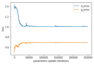
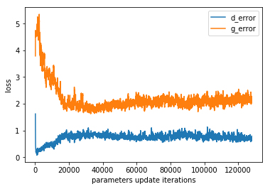
The loss from the generator and discriminator look much better:

CVAE

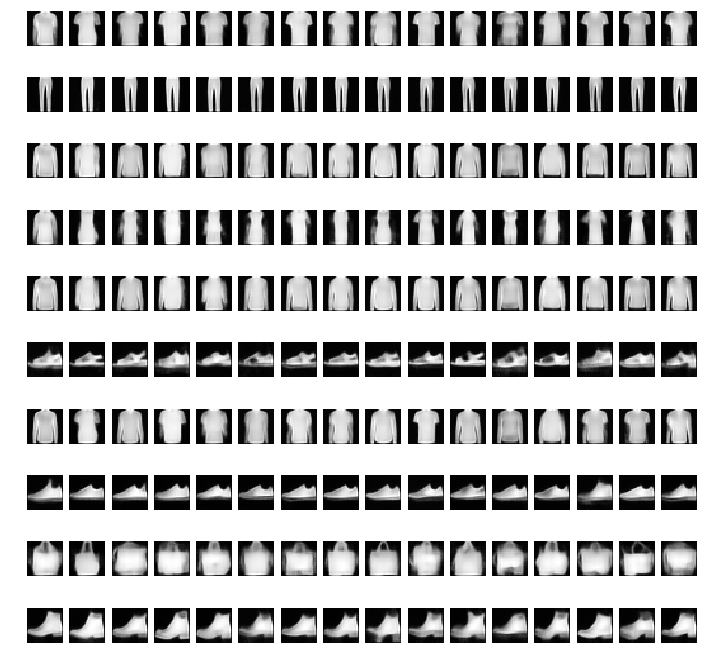
CVAE has a similar issue as DCGAN. The architecture I used for MNIST does not work for CIFAR10 dataset. I use a similar architecture used in DCGAN for CVAE model. Here are the results (after the model is converged):

There are 10 classes, but I will just plot the generated images from the first 3 classes (airplane, automobile, and bird):

Generated airplane Image using CVAE

 

Generated automobile Image using CVAE

Generated bird Image using CVAE

Although the generated images show that CVAE learns *something* but it does not learn conditional probability . My thought is that there are too many variations even between images within the same class, it can be challenging for the model to learn to draw a bird by simply observing a picture of birds alone. I find it is interesting to be able to conditional generate images. This is something I will explore further in the coming month.

Conclusion:

I have just entered the art (dark) side of the deep learning. Finding the right architecture is painful and can be frustrating. Training GANs requires a few tricks to make it work. For example, I have to use SDG to train the discriminator and use ADAM to train the generator. There is no formula for the right architecture and I hope one day we will understand deep neural nets better!

On the other hand, VAE does not generate a sharp image compared to GAN. There are many works that proposed an extension to VAE so it can generate a sharper image. That is something I will explore later as well.

Cheers!

 

 

Day 8: Move away from MNIST datasets

The MNIST dataset is too easy and can be distinguished by one pixel.

Ian Goodfellow wants people to move away from MNIST.

Instead of moving on to harder datasets than MNIST, the ML community is studying it more than ever. Even proportional to other datasets https://t.co/TAo52VC1Fg

— Ian Goodfellow (@goodfellow_ian) April 13, 2017

Francois, the Keras’s author, also advocates people to use CIFAR10 instead of MNIST:

Many good ideas will not work well on MNIST (e.g. batch norm). Inversely many bad ideas may work on MNIST and no transfer to real CV.

— François Chollet (@fchollet) April 13, 2017

No problem! I will rerun my experiments on FashionMNIST, EMNIST, CIFAR10, and STL. I will skip the SVHN dataset because the original CVAE paper already shows that SVHN works on CVAE model. For this post, I will just work on FashionMNIST and EMNIST.

CVAE model

FashionMNIST:

CVAE: Sample 16 images from each category using the same latent vectors. Each row is a category, each column is one unique latent vector of 64 dimensions.

In FashionMNIST, CVAE has a harder time distinguishing a pullover from a coat. The sneaker and sandal are also hardly distinguishable. It shows that CVAE is not so good at capturing the fine-grained detail.

EMNIST

I hardly recognize anything from here. CVAE does quite poorly here.

If CVAE does not do well, how does GANs perform on FashionMNIST and EMNIST?

DCGAN

Here are the 20 images sampled from the generator after training for 500 epochs for each dataset.

FashionMNIST:

The generated images from this dataset are somewhat okay but not great. I can still be able to tell the category of each image. Some images are not complete and some clothes look like they have a hole. The generated images are completely different from VAE. VAE is able to preserve the over the structure of the images but GANs seems to be able to take care of all the little details. The combination of the two’s could be interesting.

EMNIST

For EMNIST dataset, I can hardly recognize anything. However, EMNIST dataset itself is already difficult even for me to distinguish each letter. I can either add more capacity to the model or work on stabilizing the GAN. Currently, the discriminator’s loss goes to 0 which looks like a failure mode.

What is next:

I want to work on the color images and see how each model performs on these datasets such as CIFAR10, STL, or SVHN.

Day 7: Conditional VAE

Limitation of Vanilla VAE

Variational autoencoder (VAE) is one of the simplest deep generative models. The implementation is almost similar to a standard autoencoder, it is fast to train, and generate reasonable results.

Although VAE may not sound as sexy as GANs or is not as powerful as an autoregressive model, this model has a probabilistic perspective which can be useful for model interpretation and extensions.

But a vanilla VAE is notorious for generating a blurry image:

16 sample images from a Vanilla VAE. Each column is one unique image and each row is the epoch. Each row represents epoch iteration starting from epoch 0, 3, 6, 9, 12, and 15.

Even if the model has already converged, the image samples are not as clear as images generated by GANs. However, we can still recognize some digits.

However, sampling from VAE or any generative model is somewhat useless if we do not have the control of what we want. It would be nice if we can sample any digit we want.

Conditional VAE (First attempt)

The work from Diederik Kingma presents a conditional VAE [1] which combines an image label as part of the inference. Puting the math and derivation of the ELBO aside, the key change to the vanilla VAE’s architecture is to add a discriminator to classify the given MNIST digit and use this prediction as additional information to the decoder.

Ideally, if we tell the decoder that we want to generate a digit 1, the decoder should be able to generate the desired digit. Vanilla VAE does not have this information.

I extend VAE by simply adding a class vector to the decoder and hope that the decoder will learn to generate only digits from the given class.

Here is the result:

sampled images from the modified VAE whose the decoder takes both image latent vector and class vector. Each row represents one digit class, starting from digit 0 to digit 9. Each column represents one random vector. We use the same vectors but varies the class vector.

The result does not look good. All images in the first column look the same. The 9th column is the only column that each sample images are different.

KL Annealing

One technique to prevent VAE from being lazy and stop learning is to disable KL loss during the first few iterations and enable KL loss a bit later. This minor change helps the model to learn a good representation:

We can now see that the decoder can generate a correct digit. It shows that by just passing a class vector, the model can easily utilize this information.

The problem with fusing a class vector and latent vector?

The previous method concatenate vector of class vector and image latent vector before feeding to the decoder. This vector is transformed and reshape to a square matrix so that the deconvolutional layer is applicable. I found that fusing a class vector to the latent vector is a bit strange. The deconvolutional layer should expect a matrix that preserves the spatial relationship. E.g. The entries around the top right should be somewhat correlated. But the simple fusing method mentioned earlier does not seem to preserve this property. It would be interesting to see find out what other fusing strategies that can be more effective than just a vector concatenation.

Source Code

References:

[1] D. Kingma, “Semi-supervised learning with Deep Generative Models” NIPS’14 https://arxiv.org/pdf/1406.5298.pdf

Day 6: DCGAN

After I spent a few days on an autoregressive model, I want to switch my focus on GANs for the coming days. Today I worked on DCGAN [1] which is GANs that uses a deconvolution network as a generator and a convolution network as a discriminator.

Although the use of deconvolutional layers may sound straightforward, I still like some ideas of DCGAN’s architectures:

1. It does not use any max-pool at all and uses a strided convolutional layers to down-sampling instead. The use of multiple convolutional layers for down-sampling was proposed by [2].
2. It uses a deconvolutional layer as part of the generator by slowly double the number of channels until it reaches the desired image dimensions.
3. This is a subtle idea. It uses LeakyReLU instead of ReLU.

I modified my Vanilla GAN by replacing the generator and discriminator with conv and deconv layers.

We randomly select 16 random vectors with a dimension of 64 drawn from a normal distribution. Each column represents one unique vector. Each row represents the number of epochs.

Sampled digits generated by the generator. Each row represents the number of epoch. From top to bottom: epoch 10, 50, 100, 150, and 200. We can see that the more epochs, the better image quality.

DCGAN generates much better image quality than Vanilla GAN. Hence, convolutional and deconvolutional layers give representation and classification power to the models.

Loss Plot

To be honest, the loss does not look good to me. I expected the loss from the generator slowly decays overtimes but that is not the case here. It seems that the discriminator performs a binary classification extremely well. This could be bad for the generator since it will never receive a positive signal, but only negative signals. The better training strategy will be explored in my future study.

Closing

DCGAN is a solid work because the generated images are significantly better than Vanilla GANs. This simple model architecture is more practical and will have a long-lasting impact than a sophisticated and complex model.

Code

References:

[1] DCGAN original paper

[2] Striving For Simplicity: The All Convolutional Net  (ICLR’15)

 

Day 5: MADE – Mask Autoencoder

The main problem with NADE is that it is extremely slow to train and sample. When training on a MNIST digit, we need to compute log probability one pixel sequentially. Same goes for sampling a MNIST digit.

MADE – Mask Autoencoder [1] proposes a clever solution to speed up an autoregressive model. The key insight is that an autoregressive model is a special case of an autoencoder. By removing a weight carefully, one can convert an autoencoder to an autoregressive model. The weight removal is done through mask operations.

I used the implementation from [2] and trained MADE with a single layer of 500 hidden units on a binary MNIST dataset. I sample each image by first generating a random binary image, feed it to the MADE, then sample the first pixel. Then, I update the first-pixel value of the random binary vector. I then pass this random vector to the MADE again and so on.

Here are sampled images:

They look pretty bad! I barely notice a digit 7. This makes me wondered if a single layer MADE is not strong enough or the way I sample an image is not correct.

The strength of MADE is that training is very fast. This contribution alone makes it possible to train a large autoregressive model. I really like this paper.

References:

[1] https://arxiv.org/pdf/1502.03509v2.pdf

[2] https://github.com/karpathy/pytorch-made

 

Day 4: NADE (revisit)

Before I dive into some advance autoregressive models, I want to step back and implement NADE model proposed by Hugo et al [1]. Last year I wrote a blog post about this model but never implement the model. Hence, I will dedicate my day 4 on implementing NADE model.

The autoregressive model is similar to RNN. It is a sequential model and assumes that the current input depends on the previous inputs.

Then, the hidden state can be computed by a shared weight variable W:

Then, we compute the log-likelihood as follows:

NADE shares weight parameters so it only has one neural nets to transform the sequential data into a series of hidden variables.

However, training and sampling data from NADE are very slow. For training and sampling, we need to sequentially compute each hidden variable. This is extremely slow even for a small image such as MNIST (32×32). The recent work such as Mask Autoencoder [2] has addressed this slow training issue.

Code

References:

[1] http://proceedings.mlr.press/v15/larochelle11a/larochelle11a.pdf

[2] https://arxiv.org/abs/1502.03509

Day 3: ICA with gradient ascent

I have been trying to implement Andrew Ng’s ICA but always get a numerical error. So I have found that computing a log determinant of a matrix can be tricky and leads to numerical error.

Another ICA’s algorithm is from Shireen Elhabian and Aly Farag. I found this algorithm is more numerical stable than the Andrew Ng’s method.

I have found the code that implements both methods and I reused the author’s code to perform blind source separation task on the toy data.

Here are the results:

Original Signals

Mixed Signals (Observed Signals) 

Recovered Signals using FastICA

Recovered Signals using PCA

Recovered Signals using Andrew Ng’s method

Recovered Signals using Shireen’s method

FastICA performs extremely well on the toy data. Andrew Ng’s method is very sensitive to the learning rate and does not perform well compared to Shireen’s method. Shireen’s method produces the better recovered signals, at least for this toy data.

Lesson Learned:

I attempted to use pyTorch to implement ICA and found very difficult to get a good result due to the numerical instability. The log-determinant term is troublesome and I have spent a few days trying to understand the insight of the determinant of a matrix. It is always a good idea to look into math to get a better insight.

I think one serious drawback with the change variable method is the need to compute the determinant of the weight matrix. I found that the author of RealNVP’s paper designs the neural network so that the weight matrix is a lower-triangular matrix in which the determinant is just a product of the diagonal entries.

ICA is a linear model so it won’t do well on the complex data. Finally, to train the model using gradient descent can be tricky since some maximum-likelihood models are prone to a numerical instability.

[code]

 

 

 

 

Day 2: Independent Component Analysis (ICA)

Independent Component Analysis (ICA) is one of the topics that I haven’t spent enough times playing with it. My 2nd and 3rd days will be focused on this topic starting from the intuition and ending with implementation.

I found this tutorial extremely helpful: ICA Tutorial and cs229_note

Overview

ICA is one of the matrix factorization algorithms. We are given a mixing model:

Where we only observe a mixture x, and we need to estimate a mixing matrix A and independent component s.

This mixing model is a generative model because we need to draw multiple independent components and mix them up with mixing matrix A to generate mixture x’s.

The intuition of solving ICA is to make s as least-gaussian as much as possible. When s is Gaussian, it is impossible to estimate mixing matrix A because the joint distribution is also Gaussian and does not contain any information about A.

There are many ways to solve ICA, but I think the easiest one (with less math and statistic) is the maximum likelihood method.

Ideally, we want to perform the following optimization:

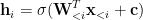
But we don’t know . However, if we know the density function of s, then we can use the change of variable technique to derive .

• First, we know that each s has to be independent, hence .
• We can compute s by .
• The density function of x is: . Note the determinant term.
• The log-likelihood is then defined as:

We want to find that maximize this log-likelihood function.

BUT we do not know !

If we have enough knowledge about s, we might be able to estimate . But one simple approximation is to just pick some non-Gaussian cdf for . Remember, we can’t choose Gaussian, otherwise, ICA won’t work [1].

We pick a sigmoid function as the CDF for [2]. Thus, .

Finally, we apply the gradient descend to solve for .

Note: It is important to know that the maximum likelihood is just one of the algorithms to solve ICA problem. There are many other interesting algorithms such as FastICA, which is probably more robust than the maximum-likelihood approach.

References:

[1] ICA Tutorial

[2] cs229_note

Day 1: Vanilla GANs

Since my internship will be over in a few days, I took a challenge from Siraj Ravel for 100MLCodingChallenge and plan to write a blog and implement on whatever topics or papers that I like. This will be fun.

For the first day, I will tackle GANs. I know about GANs for a few years but never get a chance to implement it. I am a huge fan of variational autoencoder so I was a bit bias toward a probabilistic model. But the main drawback of VAE is its dependency on the reconstruction error, which may not be a good loss criterion for some interesting problems.

I implemented a simple GANs based on a simple feedforward neural network. According to the loss plot, it seems to me that my implementation of GANs working. The loss of discriminator slowly increases while the loss from the generator slowly decreases overtimes.

I also sampled 16 images from the random uniform noise. We can see that the image quality is getting better and better overtimes as well.

10 epochs

50 epochs

100 epochs

150 epochs

200 epochs

That is it for my first day of the challenge. It will be a fun journal in the coming month.

code