Deep Autoregressive Network (ICML’14)

This is one of the early paper on generative modeling. This work was on arXiv since Oct 2013 before the reparameterization trick has been popularized [2, 3]. It is interesting to look back and see the challenge of training the model with stochastic layers.

Model Architecture

Deep Autoregressive Network (DARN) is a flexible deep generative model with the following architecture features: First, its stochastic layer is stackable. This improves representational power. Second, the deterministic layers can be inserted between the stochastic layers to add complexity to the model.  Third, the generative model such as NADE and EoNADE can be used instead of the simple linear autoregressive. This also improves the representational power.
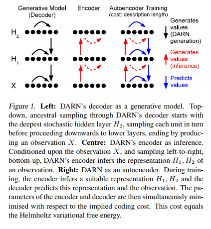
 

Darn

The main difference from VAE [2] is that the hidden units are binary vectors (which is similar to the restricted Boltzmann machine). VAE requires a continuous vector as hidden units unless we approximate the discrete units with Gumbel-Softmax.

DARN does not assume any form of distribution on its prior p(h) or conditional distribution p(x|h) and q(h|x). The vanilla VAE assumes a standard Gaussian distribution with the diagonal covariance matrix. This could be either good or bad thing for DARN.

Sampling

Since DARN is an autoregressive model, it needs to sample one value at a time, from top hidden layer all the way down to the observed layer.

Minimum Description Length

This is my favorite section of this paper. There is a strong connection between the information theory and variational lowerbound. In EM algorithm, we use Jensen’s inequality to derive the smooth function that acts as a lowerbound of the log likelihood. Some scholars refer this lowerbound as an Evidence Lowerbound (ELBO).

This lowerbound can be derived from information theory perspective. From the Shannon’s theory, the description length is:

L(x|h) = -\log_2 p(x|h)

If h is a compressed version of x, then we need to transport h along with the residual in order to reconstruct the original message x.

The main idea is simple. The less predictable event requires more bits to encode. The shorter bits is better because we will transport fewer bits over the wire. Hence, we want to minimize the description length of the following message x:

L(x) = \sum_h q(h|x)(L(h) + L(x|h))

The q(h|x) is an encode probability of h. The description length of the representation h is defined as:

L(h) = -log_2 p(h) + \log_2 q(h|x)

Finally, the entire description length or Helmholtz variational free energy is:

L(x) = -sum_h q(h|x)(\log_2 p(x,h) - \log_2 q(h|x)) (1)

This is formula is exactly the same as the ELBO when h is a discrete value.

Learning

The variational free energy formula (1) is intractable because it requires summation over all h. DARN employs a sampling approach to learn the parameter.

The expectation term is approximated by sampling h \sim q(H|x), then now we can compute the gradient of (1). However, this approach has a high variance. The authors use a few tricks to keep variance low. (Check out the apprendix).

Closing

DARN is one of the early paper that use the stochastic layers as part of its model. Optimization through these layers posed a few challenges such as high variances from the Monte Carlo approximation.

References:

[1] Gregor, Karol, et al. “Deep autoregressive networks.” arXiv preprint arXiv:1310.8499 (2013).

[2] Kingma, Diederik P., and Max Welling. “Auto-encoding variational bayes.” arXiv preprint arXiv:1312.6114 (2013).

[3] Rezende, Danilo Jimenez, Shakir Mohamed, and Daan Wierstra. “Stochastic backpropagation and approximate inference in deep generative models.” arXiv preprint arXiv:1401.4082 (2014).

ListNet and ListMLE

I just read about Learn2Rank and stumped over the ListNet [3] and ListMLE [4]. These two models are part of Learn2Rank algorithms. The goal is to learn a score function s(d) where d is a document that will yield a high score for a relevant document but low scores for non-relevant documents.

There are three main methods to learn this score function: point-wise, pair-wise, and list-wise. Point-wise: we learn this function from one sample. Pair-wise: we learn from a pair of samples, its relationship. And List-wise: we learn from a collection of samples, its order/rank.

The main essence of ListNet and ListMLE is Plackett-Luce model. (see. [1, 2]). The PL model defines a probability distribution of objects. If we have a collection of N objects, and each object has its associated score, then we can compute the probability of seeing a particular permutation. For example, I have items {A, B, C} and scores {5, 2, 1}; then PL model defines a probability distribution of all permutation of {A, B, C}.

I will not go over its definition, but you can read more from [2]. My point is we have a function that will assign the score to every possible permutation of the collection of items.

What ListNet [3] tried to do is to model a score function as a neural network. Then, the author observes that given the ground truth, we can compute the true probability of the given permutation of the items. Then, we want to learn a score function such that it will map a raw feature (document) to a score. The key idea is the probability distribution calculated from the score function should be as similar as the true probability distribution of all permutation based on the ground truth. They use KL divergence to measure the deviation of the learned distribution from the true distribution.

As we expect, ListNet can be expensive to train because we need to compute all possible permutations. Thus, people approximate the permutation by only calculate up to K permutations. K can be 1, 5, 10, 20, or 50, whatever you think is a good number.

ListMLE [4] is even a simpler model. Minimizing loss based on KL divergence is still a computational expensive. Instead, they just want to maximize the probability of the observed permutation directly. If we are given a ground truth that ‘A, B, C’ is the best permutation, then P( ABC) should have the highest probability. Then they train a neural network to learn a score function that will give a score that will satisfy this objective function.

References:

[1] Plackett, R. (1975). The analysis of permutations. Applied Stat, 24, 193-202.

[2] Guiver, John, and Edward Snelson. “Bayesian inference for Plackett-Luce ranking models.” proceedings of the 26th annual international conference on machine learning. ACM, 2009.

[3] Cao, Zhe, et al. “Learning to rank: from pairwise approach to listwise approach.” Proceedings of the 24th international conference on Machine learning. ACM, 2007.
APA

[4] Xia, Fen, et al. “Listwise approach to learning to rank: theory and algorithm.” Proceedings of the 25th international conference on Machine learning. ACM, 2008.
APA

Review some Information Theory

Here are my note on some concepts from self-study on Information Theory:

The Shannon information content:

h(x) = \log_2 \frac{1}{p(x)}

This is a measurement of the information content of the event x = a. For example, when we flip a coin, an event of landing a head is 0.5, then h(x=’head’) = 1. It means that we only need one bit for this event. E.g. If we landed a tail, we know that it won’t be a head. One bit is sufficient.

Entropy: an average of Shannon information:

H(X) = -\sum_x p(x) \log_2 p(x)  = E[- \log_2 p(x) ]

We consider all events and average out all the Shannon information. Entropy can be thought as an uncertainty. The higher entropy, the more uncertainty of the event. This implies that the Entropy will be maximum when p(x) is a uniform distribution since we can’t make any prediction.

The Relative entropy (KL Divergence)

KL(P||Q) = \sum_x p(x) \log_2 \frac{p(x)}{q(x)} = E[\log_2 \frac{p(x)}{q(x)}]

KL(P||Q) is always non-negative (Check Gibbs’ inequality). This term will show up often in many machine learning models. It measures how much distribution q(x) diverges from p(x).

The Conditional entropy of X given Y:

This is an average uncertainty that remains about x when y is known. If I know y, then how much I still don’t know about x.

H(X|Y=b_k) = - \sum p(x|y=b_k) \log_2 p(x|y=b_k)

If we average over y:

$latext H(X|Y) = \sum_y p(y) [-\sum_x p(x|y) \log_2 p(x|y) ] = -sum_{x,y} p(x,y) \log p(x|y) $

Chain rule: 

h(x,y) = h(x) + h(y|x)

Information content of x and y is the information content of x plus information coent of y given x.

Entropy Chain rule:

H(X,Y) = H(x) + H(Y|X)

An uncertainty about X and Y is the uncertainty of X plus uncertainty of Y given X.

Mutual Information:

This term appears often in information retrieval and some machine learning models. This term measures the average reduction in uncertainty about x that results from learning the value of y. E.g. How much I will learn about x once I know about y ? What is an average amount of information that y conveys about x?

I(X; Y) = H(X) - H(X|Y)

I(X; Y) = I(Y; X) \ge 0

When we add more data, we always decrease uncertainty.

H(X,Y) \le H(X) + H(Y)

H(Y|X) = H(X,Y) - H(X) \le H(Y) + H(X) - H(X) \le H(Y)

References:

[1] MacKay, David JC. Information theory, inference and learning algorithms. Cambridge university press, 2003.