Paper Reading: Semantic Hashing using Tags and Topic Modeling (SIGIR13)

This paper is similar to collaborative topic modeling. They also mentioned that in their paper. The main difference is they train LDA offline so the topic distribution is not affected by tagging (supervisory signals).

From probabilistic perspective, it is variant of CTM:

Train topic model offline.

  1. For each doc y_j in Corpus:
    1. Draw latent offset, e ~ Gaussian(0, 1)
    2. Draw document latent, y ~ e + topic(y)
  2. For each tag u_i:
    1. Draw tag, u_i, from Gaussian(0, 1)
  3. For each doc y_j and tag u_i:
    1. Draw a document label, t_{i,j} ~ Gaussian( u_i * y_j , confidence)

I think the confidence matrix that they create is simply a fixed variance.

From matrix factorization perspective:
1. They factor a tagging matrix: T = U * Y
2. Add regularizer || U ||^2 to keep U small since U is drawn from Gaussian(0,1).
3. Add regularizer that penalizes when Y is deviate from a topic(Y).

Their binarization from Y to hashcode is very straight forward.

Based on my analysis, there are a lot of rooms to improve:
1. adding non-linearity to matrix factorization, hash code function, and binarization function.
2. tagging uncertainty is learned from the data (instead of fixed variances).
3. tags (supervisory signal) can be correlated ( so document without tag t, can still have a high probability for tag t, if similar tag s appears in the doc.
4. jointly learn a topic model.
References

References:

[1] Wang, Qifan, Dan Zhang, and Luo Si. “Semantic hashing using tags and topic modeling.” Proceedings of the 36th international ACM SIGIR conference on Research and development in information retrieval. ACM, 2013.

Supervised Hashing for Image Retrieval (AAAI’14)

This paper proposed a supervised hashing method that learns hash codes from the images and a hash function using convolution neural network (CNN).

Ideally, it would be nice if the model can simultaneously learn a hash function from the train images and class labels. If they only set up CNN by learning a function that maps a raw image to class labels, then they won’t learn any good representation but instead learning a discriminative model.

Instead, they need to approximate hash codes for training data from the similarity matrix. Defining a matrix S_{i,j} = +1 if image i is semantically similar to image j. Otherwise, S_{i,j} = -1. Then they cleverly assume that a dot product between two hash code ( a binary vector) is approximately equivalent to +q if both vectors are similar. q is a dimension of a binary vector. The objective function then becomes a matrix factorization problem:
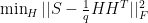
\min_{H} || S - \frac{1}{q}HH^T||_F^2 where H \in \{-1, 1 \}^{n x q}

It is very difficult to efficiently optimize the above objective function due to an integer constraint. The authors relax this restriction by allowing a range constraint, H \in [-1, 1 ]^{n x q}, which is easier to optimize using a coordinate descent algorithm using Newton direction. The contribution is the derivation of efficient optimization algorithms that learn an approximate hashcode from the range constraint.

Once hash codes from train data are obtained, the next step is to determine a hash function. They construct CNN and simultaneously learns a function that maps a raw image to an image representation (encoder) and a hash function that maps this representation to the given approximate hash codes. The author called this as the CNNH model.

By adding label information as additional output layers, now CNN needs to learn an image representation that matches the given hash codes and label matrix. This additional constraint forces the CNN to learn a shared image representation. The author called this as CNNH+ model.

The CNNH+ model has the highest MAP on MNIST, CIFAR10, and NUS_WIDE datasets.

I think using deep learning architecture is trivial but learning an approximate hash code is much more challenging when the objective function is a range constraint. The authors demonstrated that the proposed optimization method is faster and more scalable than BCD algorithm. I believe BCD [2] is the state-of-the-art method at that time.

References:

[1] Xia, Rongkai, et al. “Supervised Hashing for Image Retrieval via Image Representation Learning.” AAAI. Vol. 1. 2014.

[2] Lin, Guosheng, et al. “A general two-step approach to learning-based hashing.” Proceedings of the IEEE International Conference on Computer Vision. 2013.

Review some Information Theory

Here are my note on some concepts from self-study on Information Theory:

The Shannon information content:

h(x) = \log_2 \frac{1}{p(x)}

This is a measurement of the information content of the event x = a. For example, when we flip a coin, an event of landing a head is 0.5, then h(x=’head’) = 1. It means that we only need one bit for this event. E.g. If we landed a tail, we know that it won’t be a head. One bit is sufficient.

Entropy: an average of Shannon information:

H(X) = -\sum_x p(x) \log_2 p(x)  = E[- \log_2 p(x) ]

We consider all events and average out all the Shannon information. Entropy can be thought as an uncertainty. The higher entropy, the more uncertainty of the event. This implies that the Entropy will be maximum when p(x) is a uniform distribution since we can’t make any prediction.

The Relative entropy (KL Divergence)

KL(P||Q) = \sum_x p(x) \log_2 \frac{p(x)}{q(x)} = E[\log_2 \frac{p(x)}{q(x)}]

KL(P||Q) is always non-negative (Check Gibbs’ inequality). This term will show up often in many machine learning models. It measures how much distribution q(x) diverges from p(x).

The Conditional entropy of X given Y:

This is an average uncertainty that remains about x when y is known. If I know y, then how much I still don’t know about x.

H(X|Y=b_k) = - \sum p(x|y=b_k) \log_2 p(x|y=b_k)

If we average over y:

$latext H(X|Y) = \sum_y p(y) [-\sum_x p(x|y) \log_2 p(x|y) ] = -sum_{x,y} p(x,y) \log p(x|y) $

Chain rule: 

h(x,y) = h(x) + h(y|x)

Information content of x and y is the information content of x plus information coent of y given x.

Entropy Chain rule:

H(X,Y) = H(x) + H(Y|X)

An uncertainty about X and Y is the uncertainty of X plus uncertainty of Y given X.

Mutual Information:

This term appears often in information retrieval and some machine learning models. This term measures the average reduction in uncertainty about x that results from learning the value of y. E.g. How much I will learn about x once I know about y ? What is an average amount of information that y conveys about x?

I(X; Y) = H(X) - H(X|Y)

I(X; Y) = I(Y; X) \ge 0

When we add more data, we always decrease uncertainty.

H(X,Y) \le H(X) + H(Y)

H(Y|X) = H(X,Y) - H(X) \le H(Y) + H(X) - H(X) \le H(Y)

References:

[1] MacKay, David JC. Information theory, inference and learning algorithms. Cambridge university press, 2003.

ParagraphVec (ICML’14)

A Bag of words (BOW) is probably one the most common document representation for a textual dataset. This feature has a fixed length, which can be conveniently trained by many off the shelf machine learning algorithms. It is an intuitive representation and yet accurate enough for many practical problems. Its extension such as  TF-IDF and Okapi BM25 are competitive representation in many information retrieval tasks.

However, the word that appears early on in the sentence is probably influenced later words. This sequential information is discarded entirely by BOW representation. Another issue is it does not capture a semantic distance since it is only a word count vector.

Word2Vec is a neural network that learns a vector representation for each word in the corpus. By training the model to predict the next words in the sentence giving earlier words, the model can find a vector representation for each word. This euclidean distance between these vectors is similar to semantic distance: similar words will be nearby.

When we are working with documents, we might also want to turn each document into a fixed length vector. But how can we find a vector representation of a document? The paper by Quoc Le explained how to train the neural network to find these representations.

The idea is to think of a document vector as a document summary. Then, during the training, the model is asked to predict the next words giving earlier words in the paragraph and a document summary. For an instance, if we want to predict the next word for “We prepare food for our ___”, the next words can be “baby”, “neighbours”, “roommate”, etc. However, if we are also told that this paragraph is about a pet, then we can make a better guess that the next word is related to animals.

This model basically extends word2vec model to a longer context. It seems to work well based on their experimental results. This model shows a connection with a memory network paper: by providing an extra relevant information (summary or supporting fact), the model will make a better prediction. The difficulty is to find such a relevant and effective fact. For this work, they train the model the same way as word2vec.

References:

[1] Le, Quoc V., and Tomas Mikolov. “Distributed Representations of Sentences and Documents.” ICML. Vol. 14. 2014.

Memory Network

Today our colleague presented Memory Network [1] at our research seminar. I want to summarize my understanding on this model and compared it with other deep sequential models such as LSTM and RNNs.

In Question-Answering problem, we are given a question to a learning model, and the model will output an answer based on information and facts that it was given during the training. LSTM and Sequence-To-Sequence models are popular choices of models due to they can handle a variable length input which is common in text and these models avoid vanish gradient problem.

The Memory Network extends these earlier models by adding supporting facts as additional inputs. Intuitively, this should help the model to answer the question better because of the extra information. The model will first locate a few good facts (which is 2 sentences in this paper ) and use that as additional inputs.

Locating relevant facts is time-consuming. Thus, the authors proposed a few approximation to speeding up. The first approximation is to only search for a sentence that sharing the same word with the question. This is the fastest method but not accurate. The second approximation is to cluster all word hash and only search for sentences that have at least one word sharing the same cluster as the given question. This method is much more accurate but it is also slower.

There are a few more extensions such as adding time relation among sentences in order to answer more tricky questions.

In summing up, the memory network does not utilize all facts but instead picking a few relevant facts. The process of fact picking is inefficient. Instead, if we assign a weight to each fact, we might be able to utilize more information to answer the given question.  The following up works have exploited this idea and demonstrated better results in QA problem.

References:

[1] Weston, Jason, Sumit Chopra, and Antoine Bordes. “Memory networks.” arXiv preprint arXiv:1410.3916 (2014).

Keras: Merge vs merge

This issue gave me a headache because I did not realize that ‘Merge’ and ‘merge’ are different in Keras.

Merge is for merging layers.

merge is for merging tensors.

Without consulting with the docs and forums, there is no way I could figure this out.

References:

https://github.com/fchollet/keras/issues/2646


Entropy in Variational Inference

In Variational Inference, the evidence lowerbound (ELBO) is defined as:

\log p(x) = \log \int_z p(x, z) dz = \log E_{q(z)}[\frac{p(x,z)}{q(z)}]
>= E_{q(z)}[\log p(x, z) ]- E_{q(z)}[ \log q(z) ]

At this point, I usually pay attention to the first term, the expected log-likelihood and treat the second term, entropy, as extra baggage. It makes sense that the entropy term is less relevant especially in mean-field approximation because when the complicated approximate distribution is now just a factored of much simpler approximate distributions, q(z) = \prod_i q(z_i) , the entropy term is just a sum of entropy for each hidden variables.

The entropy term shows up again when I worked on the Variational Autoencoder formulation. The entropy term is merge with a prior and result in a relative entropy:

\log p(x) >= E_{q(z)}[\log p(x| z) ] + E_{q(z)}[\log p(z)]- E_{q(z)}[ \log q(z) ]
= E_{q(z)}[\log p(x| z) ] - D_{kl}(q(z)||p(z))

When I pay closer attention, the relative entropy represents a gap (slack) between the lowerbound and the log-likelihood. The high relative entropy means that I badly approximate the true posterior.

When I studied information theory more thoroughly, the entropy can be viewed as the uncertainty of the event of interest. The more uncertainty, the higher entropy because we need to add extra bits to encode these unknown. Then, the entropy in the ELBO could imply how useful the variational distribution. If q(z) is a uniform distribution, then it is useless because we cannot make any good prediction. Thus, we want q(z) to be less flat which automatically means more predictable and lower entropy.

I think I need to be able to look from information theory perspective to get a better sense of how things work in Variational Inference. This knowledge will definitely be helpful for my future research.