Day11-r: Gaussian Word Embedding (ICLR’14)

The order embedding paper mentioned the prior work to learn word embedding in a probabilistic way. This idea has intrigued me so I went back to read this ICLR paper. Not surprisingly, this pioneered paper was written by the student of Andrew McCallum. I am expecting a few surprises and an aha moment from this work.

This picture explains everything about Gaussian word embedding:

In word2vec, the model attempts to learn a fixed vector so that any word in the same sentence has similar vectors. The similarity among vectors is measured by the dot product. The probablistic embedding is a generalization of word2vec. Instead of learning only an embedding vector, the model needs to learn 2 vectors per word; namely mean and variance vectors.

The role of a variance is important. A common word has a higher chance to be appeared with more words than a more specific word. We could expect that a different variety of sentences formed by the common word; hence, its variance should be large.

With this intuition, the covariance matrix of word w could be estimated based on the distance among other words within the same sentence as word w:

• is a word vector found in the same sentence as word w

One problem with this estimation is that the model cannot capture many entailing relationships because some broader words are rarely appeared in the text corpus. For example, sentences “look at a dog” and “look at a bird” are far more common than sentence “look at a mammal”. The hierarchical relationship between mammal and dog could not be learned by this model.

Energy-based learning approach (EBM)

This learning framwork is a generalization of a probabilistic model. The probablistic model needs to “stick” with a probabilistic (normalized) distribution, but the energy-based model does not have to. In sum, in EMB framework, we first define a compatible function between a pair of words and use a gradient-based inference to keep the “energy” or score output by the compatible function as small as possible. One key advantage of EBM is its ability to incorporate a latent variable, which is something that can’t be done directly using feedforward networks. For a sake of this post, you will find many resources on EBM approach.

Compatible Function

This paper use an inner product between two Gaussian distributions as a similarity measurement, which is defined as:

To train the compatible function, the authors depend on log-likelihood estimation. They found that using rank loss or ratios of densities are less interpretable and possibly log-likelihood has a better numerical stability.

Another way to train the model is to use KL divergence as the distance measure. I am not sure if using KL divergence (an asymmetric distance) is applicable because we can force the word w to be closer to its neighbor word but not another way around. I guess when it comes to training the deep learning model, we don’t have to be too strict about some mathetical conditions such as the distance metric.

Learning

The mean needs to be kept as small while a covariance matrix must be positive definite. One constraint is to keep each element of the diagonal to be bounded the hypercube. This can be done by enforcing each element to be bounded some pre-defined range.

Evaluation

A broader word has a higher variance than a specific word.

Entailment

As mentioned earlier, this model can somewhat learn entailment directly from the source data. But it can’t learn all word relationships.

In sum:

It is obvious that the proposed model probably does not work well in the industry. But this paper provides a probabilstic perspective of word embedding. Indeed, this is an interesting paper. I always enjoy reading this paper greatly.

Reference:

• https://arxiv.org/pdf/1412.6623.pdf

Day10-r: Hierarchical Density Order Embeddings (ICLR’18)

Motivation:

The motivation of this paper is really interesting. Can we capture entailment relationships from the text corpus? For instance, not only do we learn the word representation, but can we also learn a hierarchical relationship among the words? A word such as “object” or “animal” shall be broader than the word “house” or “cat”.

Contributions:

• a new loss function
• a distance metric
• graph-based schemes to select negative samples.

Observation:

The author observed that a more specific word can be substituted by a broader word. For example, in the sentence: “I like iced tea”, the word “tea” can be replaced by “beverages”. The new sentence becomes “I like iced beverages”. The meaning of the sentence remains the same. This observation shows that a broader not only can be substituted but also its probability density should have a higher variance because it can be used in many contexts.

Key concepts:

• Notations:
  • for words a and b, a <- b means that every instance of a is also an instance of b, but not the otherway around.
  • then, we define the notation (a, b) which indicates that a is a hypernym of b; in contrast, b is a hyponym of a.
  • e.g. insect <- animal and animal <- organism
• Partial order:
  • the density f is more specific than a density g if f is “encompassed” in g.
  • basically, there exists x such that f(x) > n and g(x) > n. It will easier to understand this by looking at Figure 2 from the original paper.

Soft Encapsulation Orders

We can measure the order violation – basically, we count the number of items in f that violates the partial order criteria. Meaning that, how many items in set {x: f(x) > n} that is not in {x: g(x) > n}. However, this operation is difficult to evaluate. The author uses the modified KL divergence to softly estimate the order violation.

The standard KL divergence does not correctly represent the order violation. Hence, the author proposes a threshold divergence:

Loss function:

• there are two terms:
  • minimize the penalty between a true relationship pair d(u, v)
  • pushing the penalty for the negative sample (u’, v’)
  • loss =

Selecting Negative Samples

• use a graph-based methods to select negative samples.
• Method S1: replace a true hpyernym pair (u,v) with either (u,v’) or (u’,v) where u’ and v’ are randomly sampled from a uniform distribution.
• Method S2: use (v, u) if (u,v) is a true relationship pair.
• Method S3:
  • A(w) denoates all descendants of w in the training set, including w
  • randomly sample w that has at least 2 descendants and randomly select a descenant
  • then, randomly select
  • use the random neighbor par (v,u) as a negative sample.
• Method S4:
  • Same as S3 but we sample $\latex v \in A(w) – A(u) – {w}$

Summary:

This is one of my favorite papers. I really like the intuition described by the author. I haven’t explored Gaussian Embeddings on the industry dataset yet. This is something I would love to try!

References:

• https://arxiv.org/pdf/1804.09843.pdf

Day9-r: ANCE – Approximate nearest neighbor Negative Contrastive Learning (ICLR’21)

This paper proposes an effective method for sampling negative examples. They claim that their method improves the effectiveness of the dense-based retrieval model.

Local in-batch negatives are not helpful for training the dense-based retrieval model

The authors argue that the local in-batch negative fails to sample the negative examples that are hardly distinguished from the positive example. The argument starts with the batch size tends to be much smaller than the corpus size. Moreover, the number of hard negative examples is even smaller; therefore, the chance that the in-batch negative sampling will pick these hard negatives is extremely low and close to zero.

The Negative Sampling method

The negative sampling method is surprisingly intuitive. The authors use the current retrieval model to build the ANN index offline then retrieve the list of items for each query in the mini-batch from the ANN index. Any item that is not part of the positive examples will be treated as a negative example.

The challenge with this approach is to build the ANN index and retrieve the items during the training. The index building process could take a large chunk of training time. The authors opt to build the new ANN index for every m epochs. Specifically, for every m epochs, the current model checkpoint will be used to create new item vectors and these vectors will be indexed.

My thoughts:

I felt this approach could make the model overfit to the train data. However, according to the MSMACRO leaderboard (https://microsoft.github.io/MSMARCO-Document-Ranking-Submissions/leaderboard/), many top 15 models utilize the ANCE learning. This concludes that ANCE learning is an effective method for sampling a hard negative example.

Reference:

• https://arxiv.org/pdf/2007.00808.pdf

Day 6: DCGAN

After I spent a few days on an autoregressive model, I want to switch my focus on GANs for the coming days. Today I worked on DCGAN [1] which is GANs that uses a deconvolution network as a generator and a convolution network as a discriminator.

Although the use of deconvolutional layers may sound straightforward, I still like some ideas of DCGAN’s architectures:

1. It does not use any max-pool at all and uses a strided convolutional layers to down-sampling instead. The use of multiple convolutional layers for down-sampling was proposed by [2].
2. It uses a deconvolutional layer as part of the generator by slowly double the number of channels until it reaches the desired image dimensions.
3. This is a subtle idea. It uses LeakyReLU instead of ReLU.

I modified my Vanilla GAN by replacing the generator and discriminator with conv and deconv layers.

We randomly select 16 random vectors with a dimension of 64 drawn from a normal distribution. Each column represents one unique vector. Each row represents the number of epochs.

Sampled digits generated by the generator. Each row represents the number of epoch. From top to bottom: epoch 10, 50, 100, 150, and 200. We can see that the more epochs, the better image quality.

DCGAN generates much better image quality than Vanilla GAN. Hence, convolutional and deconvolutional layers give representation and classification power to the models.

Loss Plot

To be honest, the loss does not look good to me. I expected the loss from the generator slowly decays overtimes but that is not the case here. It seems that the discriminator performs a binary classification extremely well. This could be bad for the generator since it will never receive a positive signal, but only negative signals. The better training strategy will be explored in my future study.

Closing

DCGAN is a solid work because the generated images are significantly better than Vanilla GANs. This simple model architecture is more practical and will have a long-lasting impact than a sophisticated and complex model.

Code

References:

[1] DCGAN original paper

[2] Striving For Simplicity: The All Convolutional Net  (ICLR’15)

 

Generating images from captions with attention (ICLR’16)

Overview

This work extends the original DRAW paper [2] to generate images given captions. We can treat this model as conditional DRAW. That is we model a conditional probability of The additional textual data controls where to read and write the image.

AlignDRAW

Generating images from text descriptions is a structure prediction task. That is given a sequence of words, we want to generate an image. Although AlignDRAW has borrowed the same approach as DRAW by combining progressive refinement with attention, incorporating text sequence is their contribution.

The latent variable in DRAW model is sampled from spherical Gaussians, where its mean and variance are functions of the current hidden state of the encoder, e.g. . However, AlignDRAW adds dependency between latent variables: .

During the image generation, DRAW iteratively samples a latent variable from a prior , but AlignDRAW will draw from . It means that there is a dependency between each latent vector in AlignDRAW model.

Align Operator

The input caption is fed to the BI-Directional RNN. Each output from each time-step needs to be aligned with the current drawing patch. Attention weight is then learned from caption representation up to k words and the current hidden state of the decoder . Finally, compute the weight average of all hidden state of the language model to obtain the caption context, . This context together with a latent vector will be fed to the LSTM decoder.

Objective Function

This model maximizes the expectation of the variational lowerbound. There are 2 terms: the data likelihood and KL loss.

Closing Thoughts

AlignDRAW uses bi-directional LSTM with attention to aligning each word context with the patches in the image. Some generated images from caption are interesting such as ‘A herd of elephants walking across a dry grass field’. The model generalizes the training data and able to generate novel images.

References:

[1] Mansimov, Elman, et al. “Generating images from captions with attention.” arXiv preprint arXiv:1511.02793 (2015).

[2] Gregor, Karol, et al. “DRAW: A recurrent neural network for image generation.” arXiv preprint arXiv:1502.04623 (2015).

Towards a Neural Statistician (ICLR2017)

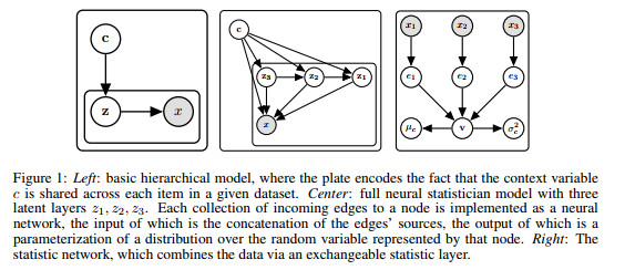
One extension of VAE is to add a hierarchy structure. In the classical VAE, the prior is drawn from a standard Gaussian distribution. We can learn this prior to the dataset so that each dataset has its own prior distribution.

The generative process is:

• Draw a dataset prior
• For each data point in the dataset
  • Draw a latent vector
  • Draw a sample

The likelihood of the dataset is:

The paper define the approximate inference network, and to optimize a variational lowerbound. The single dataset log likelihood lowerboud is:

The interesting contribution of this paper is their statistic network that approximates the posterior distribution over the context c given the dataset D. Basically, this inference network has an encoder to take each datapoint into a vector . Then, add a pool layer to aggregate into a single vector. This paper uses an element-wise mean. Finally, the final vector is used to generate parameters of a diagonal Gaussian.

This model surprisingly works well for many tasks such as topic models, transfer learning, one-shot learning, etc.

Reference:

https://arxiv.org/abs/1606.02185 (Poster ICLR 2017)

Importance Weighted Autoencoders (ICLR’16)

In a classical VAE, the ELBO is

The unbiased estimation of the gradient of is:

where

The importance weighted autoencoders has a slightly different ELBO:

The unbiased estimation of the gradient is:

Then, use the log identity:

The Monte Carlo estimation is then:

$latex \sum_{i=1}^k \tilde w_i\nabla_{\theta} \log w(\textbf{x}, \textbf{z}_i; \theta)$.

The Importance Weighted Autoencoders (IWAE) has a similar network architecture as VAE because when k = 1, the Monte Carlo estimation becomes the standard VAE.

It is unclear why IWAE is better than VAE since we can draw multiple samples from VAE to approximate its log data likelihood. The main difference is the weight function. That is why it is called Importance samples.

References:

[1] Burda, Yuri, Roger Grosse, and Ruslan Salakhutdinov. “Importance weighted autoencoders.” arXiv preprint arXiv:1509.00519 (2015).

TopicRNN : A Recurrent Neural Network with Long-Range Semantic Dependency

This paper presents a RNN-based language model that is designed to capture a long-range semantic dependency. The proposed model is a simple and elegant, and yields sensible topics.

The key insight of this work is the difference between semantic and syntax. Semantic is relating to an over structure and information of the given context. If we are given a document, its semantic is a theme or topic. Semantic is meant to capture a global meaning of the context. We need to see enough words to understand its semantics.

In contrast, a syntax is dealt with local information. The likelihood of the current word heavily depends on the preceding words. This local information depends on the word order whereas the global information does not depend on word order.

This paper points out the weakness in probabilistic topic models such as LDA such as its lack of word order, its poor performance on word prediction. If we use bigram or trigram then these higher order models become intractable. Furthermore, LDA does not model stopwords very well because LDA is based on word co-occurrence. Stopwords tend to appear everywhere because stopwords do not carry semantic information but it acts as a filler to make the language more readable. Thus, when training LDA, the stopwords are usually discarded during the preprocessing.

RNN-based language models attempt to capture sequential information. It models a word joint distribution as . The Markov assumption is necessary to keep the inference tractable. The shortcoming is the limitation of the context windows. The higher order Markov assumption makes an inferencing becomes more difficult.

The neural network language model avoids Markov assumption by modeling a conditional probability where . Basically, is a summarization of the preceding words and it uses this information to predict the current word. The RNN-based language model works pretty well but it has difficulty with long-range dependency due to the difficulty in optimization and overfitting.

Combining the advantage from both topic modeling and RNN-based is the contribution of this paper. The topic model will be used as a bias to the learned word conditional probability. They chose to make the topic vector as a bias because they don’t want to mix it up with the hidden state of RNN that includes stop words.

The model has a binary switch variable. When it encounters a stopword, the switch is off and disable a topic vector. The switch is on otherwise. The word probability is defined as follows:

The switch variable, turn on and off the topic vector .

This model is an end-to-end network, meaning that it will jointly learn topic vectors and local state from RNN. The topic vector is coupled with RNN’s state so the local dynamic from word sequence will influence the topic vector and wise verse.

RNN can be replaced with GRU or LSTM. The paper shows that using GRU yields the best perplexity on Penn Treebank (PTB) dataset. The learned representation can be used to as a feature for many tasks including sentiment analysis where we want to classify positive and negative reviews on IMDB dataset.

I found this model is simple and elegantly combine VAE with RNN. The motivation is clear and we can see why using contextual information learned from VAE will improve the quality of the representation.

reference:

https://arxiv.org/abs/1611.01702 (ICLR 2017 – Poster)

 

ICLR open review system

http://www.kdnuggets.com/2016/02/iclr-deep-learning-scientific-publishing-experiment.html