Day2-s: Hexagonal Hierarchical Spatial Index

“Pentagon is a hexagon without one side.” – Joseph Gilley

Searching on the map data is more challenging than a typical document search. Geolocation and potentially time are additional dimensions that must be considered when dealing with this complex search.

Mapping geolocation to a grid

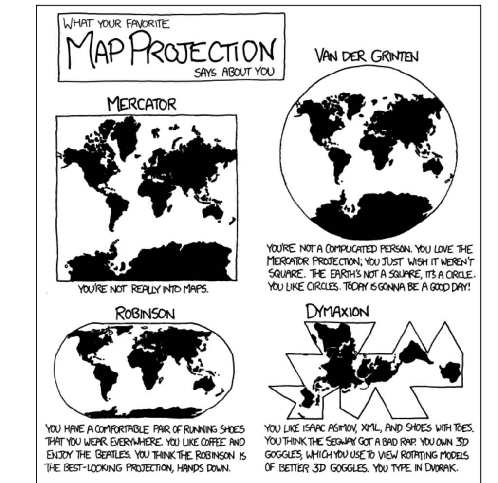
The first step is to map all locations on the earth into a 2-d space. Mathematically, it needs to map a sphere to a flat surface. There are a lot of ways to do this type of projection. They use Dymaxion projection. They use an icosahedron so that they can project a sphere to a plane. Google S3 uses a cube but Uber claims that icosahedron is a better choice.

The benefit of using the icosahedron is to reduce the distortion. The larger angle of the projection, the more distortion. Projecting on an icosahedron has the smallest angles of the projection. The orientation of the projection is also important. There is only one orientation such that all the vertices are in the water. Since the location near the vertex has the highest distortion, this orientation reduces the distortion on any land surface.

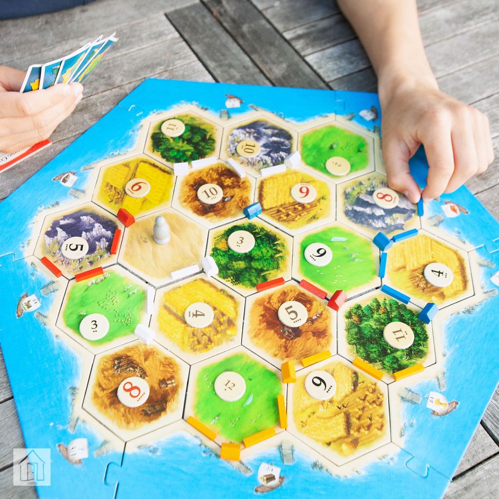
Why a hexagon is used as a tiling unit?

• neighbor traversal
  • The neighbors are always a grid that shares the same edge. It is harder to determine the neighbors using a triangle or rectangle.
• subdivision
  • It is easier to create a larger grid by composing smaller hexagons.
• distortion
  • It has less distortion compared to a rectangle.

One interesting hack is to tile the globe with hexagons but they need 12 pentagons.

Reference:

• https://eng.uber.com/h3/
• https://www.youtube.com/watch?v=ay2uwtRO3QE&t=1000s&ab_channel=UberEngineering
• XKCD Map projection: https://xkcd.com/977/

Day9-r: ANCE – Approximate nearest neighbor Negative Contrastive Learning (ICLR’21)

This paper proposes an effective method for sampling negative examples. They claim that their method improves the effectiveness of the dense-based retrieval model.

Local in-batch negatives are not helpful for training the dense-based retrieval model

The authors argue that the local in-batch negative fails to sample the negative examples that are hardly distinguished from the positive example. The argument starts with the batch size tends to be much smaller than the corpus size. Moreover, the number of hard negative examples is even smaller; therefore, the chance that the in-batch negative sampling will pick these hard negatives is extremely low and close to zero.

The Negative Sampling method

The negative sampling method is surprisingly intuitive. The authors use the current retrieval model to build the ANN index offline then retrieve the list of items for each query in the mini-batch from the ANN index. Any item that is not part of the positive examples will be treated as a negative example.

The challenge with this approach is to build the ANN index and retrieve the items during the training. The index building process could take a large chunk of training time. The authors opt to build the new ANN index for every m epochs. Specifically, for every m epochs, the current model checkpoint will be used to create new item vectors and these vectors will be indexed.

My thoughts:

I felt this approach could make the model overfit to the train data. However, according to the MSMACRO leaderboard (https://microsoft.github.io/MSMARCO-Document-Ranking-Submissions/leaderboard/), many top 15 models utilize the ANCE learning. This concludes that ANCE learning is an effective method for sampling a hard negative example.

Reference:

• https://arxiv.org/pdf/2007.00808.pdf

Day5-r: Doc2Query

The idea of this approach is to expand the document with the predicted query terms. The original work trained the LSTM-based seq2seq model to learn the generate a query from the given pair of document and query. Later, the author trained the Bert-based T5 model and demonstrated the improved in the recall on MSMACRO dataset.

To understand a little deeper, Doc2Query adds more terms into the original document. This is an indirect way to modify the term frequency in the document. The later study shows that 60% of the generated terms are found in the input document. It means that Doc2Query can find the relevant terms. Another interesting finding is that another 40% of generated query term are not found in the input document. This demonstrates that Doc2Query addresses the vocabulary gap, which is a common problem in the IR task.

I like this work due to its simplicity and effectiveness for the retrieval task.

Reference:

• https://arxiv.org/pdf/1904.08375.pdf

Day4-r: Birch

One major limitation of monoBert is its inability to process a long document. monoBert truncates the concatenation of query and document tokens within 512 tokens. This could be a sub-optimal when we are dealing with a long document. There are many works recently propose a solution for applying Bert for a long document.

For this paper, the approach proposed for allowing Bert to process a long document is somewhat unexpected. The authors simply do not let Bert process a long document at all. Instead, they treat each sentence within the same document as an individual document. By doing this, they can avoid pass a long document to Bert model.

The first insight that the authors exploit is that only a few sentences in the documents are sufficient to represent the entire document (at least for a passage ranking task). This is somewhat surprising because we could end up losing a lot of information from the document. The way they compute the document score for the given query is to use the Bert to score all pair of (query, sentence), then pick the top 3 pairs with the highest scores, then the sum of these scores is the relevant score for this long document. This is a pretty simple idea and it works.

Another finding that the authors found has to do with the transferring. They found that Bert model is effective as transferring the knowledges from one domain to another. They found that by fine-tuning the Bert with Twitter ranking dataset, then fine-tuning one more time with the domain-specific task gives a significant boost in the performance. This demonstrates how well Bert can capture the common knowledge between two datasets.

Reference:

• https://www.aclweb.org/anthology/D19-3004.pdf

Day3-r: Doc Ranking with a Pretrained Seq2Seq model

This work proposes a ranking model by turning the ranking problem into a seq-2-seq problem. This work utilizes the seq-2-seq model, T5, as the pretrained model.

The previous work, monoBert, uses a pre-trained Bert’s encoder to learn the embedding of the [CLS] token. Then, this vector is passed to the feed-forward layer which outputs the relevant score.

This work does not use [CLS] token but instead passes a sequence of output vectors from the encoder to the Bert decoder to predict the target word. The target word is “true” or “false” tokens. The output token space still covers all possible tokens. During the inference, the authors use the logits from “true” and “false” tokens and apply softmax on these two logits. Then, rank the documents based on the probability of the “true” token.

One of the most notable results is that this model is very robust on the small training data. We could argue that this rank model based on the T5 is a larger model compared to the monoBert.

Update: (April 26, 2021)

After I read the original paper that proposes T5 model, T5 model is also trained on the much larger dataset.

Reference:

• https://arxiv.org/pdf/2003.06713.pdf

Day2-r: duoBert

From the paper from day 1, it shows that a simple Bert architecture can outperform the state-of-the-arts neural IR models on re-ranking task. The natural extension of the previous work is to change the loss function from point-wise loss to pair-wise loss. They called the pair-wise model as duoBert and the original point-wise model as monoBert. But this extension would’t be interesting enough.

Hence, the authors cascades the BM25 with monoBert and duoBert as a multi-stage ranking. This approach is well-known in the industry because duoBert is too slow to rank all documents. It is more latency-friendly to employ a lesser complex model to filter out uninteresting items so that duoBert will only focus on interesting items.

By cascading BM25, monoBert, and duoBert all together, the authors show that they can achieve the best recall. Here is the architecture:

Multi-stage ranking: BM25 -> monoBert -> duoBert

What I found from this paper that might be useful is the aggregation function. In the duoBert, the model computes the relevant score by comparing two input documents, p(d1, d2). In order to rank multiple documents, the model needs to compute the relevant scores for all possible pairs of documents. Specifically, the They tried different aggregation function and shows that summing and binary function work quite well.

Reference:

• https://arxiv.org/pdf/1910.14424.pdf

Day1-r: Passage Reranking with Bert

This is one of the early works that applies Bert architecture to the search problem. In search problem, there are two main stages: retrieval and re-ranking stages. The retrieval stage deals with retrieve relevant documents from a large candidate set. This stage must be fast and efficient but does not need to be accurate. The reranking stage is more concerned with rank the small set of documents. This stage allows the more computational expensive model such as Bert. This paper focuses on the re-ranking stage.

Bert has made a significantly impact to NLP and IR research communities. This paper proposes a simple search architecture for document re-ranking.

The architecture is as follows:

The model architecture proposed by this work

The authors fine-tune the Bert model on MS MACRO (400M tuples of a query, relevant and non-relevant passage) and TREC-CAR (2.3M queries) datasets using the cross-entropy loss as an objective function.

The results look promising:

This work demonstrates that even we apply the relevant/non-relevant passage data directly to the Bert model, the model has already outperformed many state-of-the-arts neural ranking models.

The main drawback could be that this model is only applicable for the reranking stage because it has to compute the relevant score for all documents which might be too slow when we are dealing with a large number of documents (1M+). Hence, the number of passages to rank can be limited for any practical search application.

Reference:

[1] https://arxiv.org/pdf/1901.04085.pdf

Embedding-based Query Language Models (ICTIR’16)

This paper proposes a more accurate query language model for query expansion task based on word embedding.

The key contribution is their observation that the cosine similarity score between the top words with the query word is not too distant from the similarity score between the 1000th word with the same query. They use a sigmoid function to amplify the similarity score.

The rest of the paper proposes two query language models.

The first model

The first model assumes the conditional independence between the query terms.

The model is:

It defines:

And

The second model

This model now assumes that query and term similarity is independent:

$latex p(w,w’|\theta_q) = p(w|w’) = \frac{\delta(w,w’)}{\sum_{w”\in V} \delta(w”, w’)}$

and the second term uses MLE to estimate the probability:

The paper also talked about the embedded-based relevance model. The existing model by the same author is now extent with the proposed embedded query language model.

References:

[1] Zamani, Hamed, and W. Bruce Croft. “Embedding-based query language models.” Proceedings of the 2016 ACM on International Conference on the Theory of Information Retrieval.

https://ciir-publications.cs.umass.edu/getpdf.php?id=1225

Pseudo-Relevance Feedback based on Matrix Factorization (CIKM’16)

This work uses pseudo-relevance feedback collections to recommend top words and their weights to the input query.

It starts with creating a document-word matrix where each row each retrieved documents and each column is term weight. The first row is the input query’s term weights. The rest of documents either come from relevant feedback or top-K retrieved documents (pseudo-relevant feedback).

Then, we perform a non-negative matrix factorization (NMF) on the matrix. The first row of the reconstructed matrix is a re-estimate query and its top m terms will be used query expansion terms.

However, this model needs to re-compute NMF for every query, this can be expensive operations. Thus, the paper recommends creating a small document-word matrix (e.g use only top 10 retrieved documents).

What makes this model stands out is that the model not only considers the words that discriminate the top documents from the collection, it only considers the relevance of those words to the original query.

I am wondered if calculate the NMF on such a small matrix will really work. The empirical results demonstrate that this idea works but its performance is not impressive. But I think using NMF for a query expansion task is a neat idea.

References:

https://ciir-publications.cs.umass.edu/getpdf.php?id=1224

A Dual Embedding Space Model for Document Ranking (WWW’16)

This paper uses word embedding learned from word2vec model to improve the text retrieval task.

In and out Matrices in Word2Vec

Word2Vec boils down to learn two sets of word embedding matrices: and . The objective function is to maximize the similarity between the source word and the target word :

should be high if both words appear in the same context window.

The relationship among word vectors in is different from . Each similar word vectors in have common semantic. For an instance, Cambridge and Oxford are both well-known university in the UK. On the other hands, The similar word vectors in share the common context. The word such as highlights, jersey, and stadium are all related to sport. This paper exploits this fact for the retrieval task.

Aboutness

The authors postulate that document’s aboutness is a key ingredient of retrieving more relevant documents.  For example, when a query word contains word ‘jersey’, the retrieved documents that contain the related words to sports context should probably be more relevant than the document that simply has synonym words such as ‘t-shirt’ or ‘cloths’. Without context information, the word such as ‘t-shirt’ can appear also in shopping context as well as sports context.

Document Retrieval Task

The goal is to find a relevant document that matches the information need. The vector space model such as BM25 scores a higher point to those documents with an exact keyword match. Although keyword matching is very accurate, it has a few flaws. It is not robust to the keyword stuffing problem where some spam website loaded with keywords that are irrelevant to the website. The vector space model cannot detect this problem.

Hence, the relevant score should reflect how well the query matches the context of the document. If the query keyword is ‘Cambridge’, the relevant context should contain words related to universities such as faculty, students, or campus. This intuition motivates the authors to use word embedding from IN matrix () for a query and word embedding from OUT matrix () for documents.

Document Representation

The document representation is a centroid (an average) of all word vectors in the documents. This area could be improved because not all words represent the document equally.

Relevant Score

Finally, to compute a relevant score between query and document, the author uses a cosine similarity between a query vector and document centroid. Furthermore, the exact matching is still important. The final model averages the score between their proposed model and BM25. This simple change yields the best NDCG score.

This paper made me re-think about the key difference between local context used in word2vec and global context used in a topic model. I hope by utilizing both information (local and global) will help us find an even more relevant documents.

References:

Click to access 1602.01137.pdf