Deep Autoregressive Network (ICML’14)

This is one of the early paper on generative modeling. This work was on arXiv since Oct 2013 before the reparameterization trick has been popularized [2, 3]. It is interesting to look back and see the challenge of training the model with stochastic layers.

Model Architecture

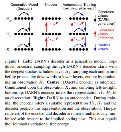
Deep Autoregressive Network (DARN) is a flexible deep generative model with the following architecture features: First, its stochastic layer is stackable. This improves representational power. Second, the deterministic layers can be inserted between the stochastic layers to add complexity to the model.  Third, the generative model such as NADE and EoNADE can be used instead of the simple linear autoregressive. This also improves the representational power.

 

The main difference from VAE [2] is that the hidden units are binary vectors (which is similar to the restricted Boltzmann machine). VAE requires a continuous vector as hidden units unless we approximate the discrete units with Gumbel-Softmax.

DARN does not assume any form of distribution on its prior or conditional distribution and . The vanilla VAE assumes a standard Gaussian distribution with the diagonal covariance matrix. This could be either good or bad thing for DARN.

Sampling

Since DARN is an autoregressive model, it needs to sample one value at a time, from top hidden layer all the way down to the observed layer.

Minimum Description Length

This is my favorite section of this paper. There is a strong connection between the information theory and variational lowerbound. In EM algorithm, we use Jensen’s inequality to derive the smooth function that acts as a lowerbound of the log likelihood. Some scholars refer this lowerbound as an Evidence Lowerbound (ELBO).

This lowerbound can be derived from information theory perspective. From the Shannon’s theory, the description length is:

If is a compressed version of , then we need to transport along with the residual in order to reconstruct the original message .

The main idea is simple. The less predictable event requires more bits to encode. The shorter bits is better because we will transport fewer bits over the wire. Hence, we want to minimize the description length of the following message :

The is an encode probability of . The description length of the representation is defined as:

Finally, the entire description length or Helmholtz variational free energy is:

This is formula is exactly the same as the ELBO when is a discrete value.

Learning

The variational free energy formula (1) is intractable because it requires summation over all . DARN employs a sampling approach to learn the parameter.

The expectation term is approximated by sampling , then now we can compute the gradient of (1). However, this approach has a high variance. The authors use a few tricks to keep variance low. (Check out the apprendix).

Closing

DARN is one of the early paper that use the stochastic layers as part of its model. Optimization through these layers posed a few challenges such as high variances from the Monte Carlo approximation.

References:

[1] Gregor, Karol, et al. “Deep autoregressive networks.” arXiv preprint arXiv:1310.8499 (2013).

[2] Kingma, Diederik P., and Max Welling. “Auto-encoding variational bayes.” arXiv preprint arXiv:1312.6114 (2013).

[3] Rezende, Danilo Jimenez, Shakir Mohamed, and Daan Wierstra. “Stochastic backpropagation and approximate inference in deep generative models.” arXiv preprint arXiv:1401.4082 (2014).

DRAW: A Recurrent Neural Network For Image Generation (ICML’15)

This paper proposes a new method for image generation by progressively improve the reconstructed image.

The previous image generation models generate the entire image by learning a sampling function (GANs), distribution over a latent vector (VAE), or generate one pixel at a time (PixelRNN, PixelCNN). Although the generated images from these models are in a good quality, these models are forced to learn a complicated and high-dimensional distribution. For example, to generate a car image, the models need to approximate the distribution of all possible cars. This is a difficult task.

(Note: I took this Figure from the original paper)

Incremental Update

Progressive refinement breaks down the complex distribution into a chain of conditional distribution:

Therefore, estimating a conditional distribution is much easier. The conditional probability is modeled by the standard LSTM.

Latent Variable

Use VAE framework helps us project the input image which has a high dimension into a low-dimensional space. Working on the smaller latent space is much easier than the original image space.

Attention Mechanism

The progressive refinement through LSTM has simplified the complex distribution through time, then the attention mechanism simplifies the spatial data into a smaller patch. The encoder and decoder now only needs to deal with a small fraction of the image instead of the image as a whole. This idea again reduces the input space by focusing on the important part of the image only.

Read and Write Operations

This part can be intimated to read at the first glance due to the use of the Gaussian filters. There are many nice blogs that described Read and Write operations with attention mechanism in detail. The main idea is the Read operation crops the input image. The Write operation draws a patch to the canvas matrix.

Closing

This is a must-read paper. The combine of progress refinement through time with attention mechanism is a nice idea to simplify the complex image distribution. This is one of the early paper that combine RNN with attention to handle the spatial data such image. I think this is an amazing accomplishment.

References:

[1] Gregor, Karol, et al. “DRAW: A recurrent neural network for image generation.” arXiv preprint arXiv:1502.04623 (2015).

 

Improved Variational Autoencoders for Text Modeling using Dilated Convolutions (ICML’17)

One of the reasons that VAE with LSTM as a decoder is less effective than LSTM language model due to the LSTM decoder ignores conditioning information from the encoder. This paper uses a dilated CNN as a decoder to improve a perplexity on held-out data.

Language Model

The language model can be modeled as:

LSTM language model use this conditional distribution to predict the next word.

By adding an additional contextual random variable [2], the language model can be expressed as:

The second model is more flexible as it explicitly model a high variation in the sequential data. Without a careful training, the VAE-based language model often degrades to a standard language model as the decoder chooses to ignore the latent variable generated by the encoder.

Dilated CNN

The authors replace LSTM decoder with Dilated CNN decoder to control the contextual capacity. That is when the convolutional kernel is large, the decoder covers longer context as it resembles an LSTM. But if the kernel becomes smaller, the model becomes more like a bag-of-word. The size of kernel controls the contextual capacity which is how much the past context we want to use to predict the current word.

Stacking Dilated CNN is crucial for a better performance because we want to exponentially increase the context windows. WaveNet [3] also uses this approach.

Conclusion

By replacing VAE with a more suitable decoder, VAE can now perform well on language model task. Since the textual sequence does not contain a lot of variation, we may not notice an obvious improvement. We may see more significant improvement in a more complex sequential data such as speech or audio signals. Also, the experimental results show that Dilated CNN is better than LSTM as a decoder but the improvement in terms of perplexity and NLL are still incremental to the standard LSTM language model. We hope to see stronger language models using VAE in the future.

References:

[1] Yang, Zichao, et al. “Improved Variational Autoencoders for Text Modeling using Dilated Convolutions.” arXiv preprint arXiv:1702.08139 (2017).

[2] Bowman, Samuel R., et al. “Generating sentences from a continuous space.” arXiv preprint arXiv:1511.06349 (2015).

[3] Oord, Aaron van den, et al. “Wavenet: A generative model for raw audio.” arXiv preprint arXiv:1609.03499 (2016).

Pixel Recurrent Neural Networks (ICML’16)

This paper proposes a novel autoregressive model to generate an image pixel by pixel. This idea makes sense since each pixel is correlated to its neighbor pixels. The same object has similar color and gradient. This idea has been exploited in an image compression such as jpeg where the color frequency does not change too frequent.

With this intuition, an autoregressive model assigns a probability of the observed sequence as For an image, each pixel is conditioned on the previous seen pixels.

A recurrent neural network such as LSTM has been an effective architecture for a sequence learning task. Hence, LSTM can be applied for an image generation task as well. There are two main challenges with using an autoregressive model for an image: first, an image is a 2-dimensional object – squeezing it to a 1-d vector will lose spatial information; second, training pixel by pixel is time-consuming and can’t be parallelized because we have to process the previous pixel before the current pixel. This paper attempts to solve these problems.

Model a color image 

Each pixel has 3 values: an intensity in the red, green, and blue channels. The conditional distribution is modified as:

Each color is conditioned on the other channels as well as the previous pixel values.

Pixels as Discrete Value

This is a neat idea. Using a discrete distribution provides more flexibility because we do not assume the shape of the distribution.

Now we will dive into the proposed architectures:

Row LSTM

When we apply LSTM on 2-dimensional input, we can first compute all the hidden states given the current pixel values and previous states. In this architecture, the previous states are the hidden states from the above rows. We can define the context window to control the amount of information to capture from the above row. If we set the context window to 3 (meaning taking the top, top-right, and top-left pixels’ hidden states):

We can parallelize this computation row by row.

Diagonal BiLSTM

One limitation of ROW LSTM is its lack of full context from the above row. By using bi-directional LSTM, this architecture can capture forward and backward dependency. Furthermore, each hidden state depends on the top-left and left hidden states:

However, the input image needs to be screwed by shifting each row by one pixel to the right, in order to parallelize this operation, column by column.

Pixel CNN

The sequential model is slow because it needs to process the previous states. Using convolutional layers to capture the spatial information is possible. But directly applying a convolutional kernel violates the autoregressive model’s assumption because the current pixel must not see the next pixel. Otherwise, we can’t generate the pixel because we will not know any incoming pixel. Hence, the mask is used to prevent the current pixel from seeing the future pixels. This trick is pretty neat.

Results

Diagonal BiLSTM has the best performance out of 3 architectures in terms of nats (negative log-likelihood) scores. The autoregressive model does not assume the low-dimensional manifold assumption and it models a conditional distribution directly. However, the computation is quite expensive for a large input.

References:

Click to access 1601.06759.pdf

A Neural Autoregressive Approach for Collaborative Filtering (ICML’16)

This paper proposed an autoregressive model for rating prediction. The idea of this paper is similar to CF-RBM for collaborative filtering problem. Instead, it replaces an RMB with NADE. Since NADE is a mean-field approximation of RBM and also CF-RBM works for collaborative filtering problem, it makes sense that NADE model is applicable for CF problem.

The NADE model aims to estimate a probability of the given sequence as The previously seen sequence of rating can be used to predict the current rating. This also implies that some early rating on the known sequence has a strong influence on the current rating. This observation made NADE a different model from RNN.

The conditional probability distribution is defined as:

The model needs to estimate a score function such that it gives a high score when a user will likely to give a rating k to an item given her previous rating history.

The score function can be seen as a dot product of a user state with an item latent vector. . The bias is an item popularity and the dot product is the similarity between the current taste of the given user to the item .

The hidden state captures the user’s current interest. It means that this model captures the change of behavior. This hidden state is defined as The function g is an activation function, c is a bias, and a matrix W is an interaction matrix that transforms the input rating vector to a item vector.

The NADE-CF can be complicated but the main idea is the same as RBM-CF. Each user will have her own NADE network. NADE-CF shares all weight parameters among all users to avoid overfitting. Further, since each weight matrix associated with a rating, some weight matrix might be updated less frequently than others. The author changes the formula to compute the hidden state (look at the eq. 9 in the original paper). This way, the rare rating matrix will be updated more often.

In order to reduce the number parameters further, the low-rank matrix approximation is applied to matrix W and V. In addition, to improve the predictability further, the ordinal cost is introduced. The idea is if the user rating item m with rating k. Her rating preference of k-1 should be higher than k-2 and so on. In other words, if a user gave a rating of 3, it is likely that she will give a rating of 2 instead of 1 because a rating of 2 is closer to a rating of 3. The ordinal cost then is modeled as a rank loss similar to the list-wise learning to rank model.

Overall, NADE-CF yields a very good performance on the popular CF data set such as Netflix and MovieLens. The model is complicated and seems to be slow. However, with ordinal cost, low-rank approximation, and its ability to have a deeper model, made this model more attractive and it might be worthwhile to investigate an autoregressive model for this particular task.

 

Autoencoding beyond pixels using a learned similarity metric (ICML’16)

One of the key components of an autoencoder is a reconstruction error. This term measures how much useful information is compressed into a learned latent vector. The common reconstruction error is based on an element-wise measurement such as a binary cross entropy for a black-and-white image or a square error between a reconstructed image and the input image.

The authors think that an element-wise measurement is not an accurate indicator of goodness of a learned latent vector. Hence, they proposed to learn a similar metric via an adversarial training. Here is how they set up the objective functions:

They use VAE to learn a latent vector of the input image. There are two loss functions in a vanilla VAE: a KL loss and a negative log data-likelihood. They replace the second loss with a new reconstruction loss function. We will talk about this new loss function in the next paragraph. Then, they have a discriminator that tries to distinguish the real input data from the generated data from the decoder of VAE. The discriminator will encourage the VAE to learn stronger encoder and decoder.

The discriminator can be decomposed into 2 parts. If it has L + 1 layers, then the first L layers is a transform function that maps the input data into a new representation. The last layer is a binary classifier. This means that if we input any input through the first L layer, we will get a new representation that is easily classified by the last layer of the discriminator. When the discriminator is very good at detecting the real input, the representation at L layer is going to be much easier to classify compared to the input data. It means that a square error between a transformed input and its transformed reconstruction input should be somewhat small when these inputs are similar.

This model has trained the same fashion as GANs; simultaneously train VAE and GANs. This idea works well for an image because the square-error is not a good metric for an image quality. This idea may work on text dataset as well because we assess the quality of the reconstructed texts based on the whole input but not collectively evaluate one word at a time.

 

References:

https://arxiv.org/abs/1512.09300

ListNet and ListMLE

I just read about Learn2Rank and stumped over the ListNet [3] and ListMLE [4]. These two models are part of Learn2Rank algorithms. The goal is to learn a score function where d is a document that will yield a high score for a relevant document but low scores for non-relevant documents.

There are three main methods to learn this score function: point-wise, pair-wise, and list-wise. Point-wise: we learn this function from one sample. Pair-wise: we learn from a pair of samples, its relationship. And List-wise: we learn from a collection of samples, its order/rank.

The main essence of ListNet and ListMLE is Plackett-Luce model. (see. [1, 2]). The PL model defines a probability distribution of objects. If we have a collection of N objects, and each object has its associated score, then we can compute the probability of seeing a particular permutation. For example, I have items {A, B, C} and scores {5, 2, 1}; then PL model defines a probability distribution of all permutation of {A, B, C}.

I will not go over its definition, but you can read more from [2]. My point is we have a function that will assign the score to every possible permutation of the collection of items.

What ListNet [3] tried to do is to model a score function as a neural network. Then, the author observes that given the ground truth, we can compute the true probability of the given permutation of the items. Then, we want to learn a score function such that it will map a raw feature (document) to a score. The key idea is the probability distribution calculated from the score function should be as similar as the true probability distribution of all permutation based on the ground truth. They use KL divergence to measure the deviation of the learned distribution from the true distribution.

As we expect, ListNet can be expensive to train because we need to compute all possible permutations. Thus, people approximate the permutation by only calculate up to K permutations. K can be 1, 5, 10, 20, or 50, whatever you think is a good number.

ListMLE [4] is even a simpler model. Minimizing loss based on KL divergence is still a computational expensive. Instead, they just want to maximize the probability of the observed permutation directly. If we are given a ground truth that ‘A, B, C’ is the best permutation, then P( ABC) should have the highest probability. Then they train a neural network to learn a score function that will give a score that will satisfy this objective function.

References:

[1] Plackett, R. (1975). The analysis of permutations. Applied Stat, 24, 193-202.

[2] Guiver, John, and Edward Snelson. “Bayesian inference for Plackett-Luce ranking models.” proceedings of the 26th annual international conference on machine learning. ACM, 2009.

[3] Cao, Zhe, et al. “Learning to rank: from pairwise approach to listwise approach.” Proceedings of the 24th international conference on Machine learning. ACM, 2007.
APA

[4] Xia, Fen, et al. “Listwise approach to learning to rank: theory and algorithm.” Proceedings of the 25th international conference on Machine learning. ACM, 2008.
APA

ParagraphVec (ICML’14)

A Bag of words (BOW) is probably one the most common document representation for a textual dataset. This feature has a fixed length, which can be conveniently trained by many off the shelf machine learning algorithms. It is an intuitive representation and yet accurate enough for many practical problems. Its extension such as  TF-IDF and Okapi BM25 are competitive representation in many information retrieval tasks.

However, the word that appears early on in the sentence is probably influenced later words. This sequential information is discarded entirely by BOW representation. Another issue is it does not capture a semantic distance since it is only a word count vector.

Word2Vec is a neural network that learns a vector representation for each word in the corpus. By training the model to predict the next words in the sentence giving earlier words, the model can find a vector representation for each word. This euclidean distance between these vectors is similar to semantic distance: similar words will be nearby.

When we are working with documents, we might also want to turn each document into a fixed length vector. But how can we find a vector representation of a document? The paper by Quoc Le explained how to train the neural network to find these representations.

The idea is to think of a document vector as a document summary. Then, during the training, the model is asked to predict the next words giving earlier words in the paragraph and a document summary. For an instance, if we want to predict the next word for “We prepare food for our ___”, the next words can be “baby”, “neighbours”, “roommate”, etc. However, if we are also told that this paragraph is about a pet, then we can make a better guess that the next word is related to animals.

This model basically extends word2vec model to a longer context. It seems to work well based on their experimental results. This model shows a connection with a memory network paper: by providing an extra relevant information (summary or supporting fact), the model will make a better prediction. The difficulty is to find such a relevant and effective fact. For this work, they train the model the same way as word2vec.

References:

[1] Le, Quoc V., and Tomas Mikolov. “Distributed Representations of Sentences and Documents.” ICML. Vol. 14. 2014.