Motivation:
The motivation of this paper is really interesting. Can we capture entailment relationships from the text corpus? For instance, not only do we learn the word representation, but can we also learn a hierarchical relationship among the words? A word such as “object” or “animal” shall be broader than the word “house” or “cat”.
Contributions:
- a new loss function
- a distance metric
- graph-based schemes to select negative samples.
Observation:
The author observed that a more specific word can be substituted by a broader word. For example, in the sentence: “I like iced tea”, the word “tea” can be replaced by “beverages”. The new sentence becomes “I like iced beverages”. The meaning of the sentence remains the same. This observation shows that a broader not only can be substituted but also its probability density should have a higher variance because it can be used in many contexts.
Key concepts:
- Notations:
- for words a and b, a <- b means that every instance of a is also an instance of b, but not the otherway around.
- then, we define the notation (a, b) which indicates that a is a hypernym of b; in contrast, b is a hyponym of a.
- e.g. insect <- animal and animal <- organism
- Partial order:
- the density f is more specific than a density g if f is “encompassed” in g.
- basically, there exists x such that f(x) > n and g(x) > n. It will easier to understand this by looking at Figure 2 from the original paper.
Soft Encapsulation Orders
We can measure the order violation – basically, we count the number of items in f that violates the partial order criteria. Meaning that, how many items in set {x: f(x) > n} that is not in {x: g(x) > n}. However, this operation is difficult to evaluate. The author uses the modified KL divergence to softly estimate the order violation.
The standard KL divergence does not correctly represent the order violation. Hence, the author proposes a threshold divergence:
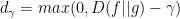
Loss function:
- there are two terms:
- minimize the penalty between a true relationship pair d(u, v)
- pushing the penalty for the negative sample (u’, v’)
- loss =

Selecting Negative Samples
- use a graph-based methods to select negative samples.
- Method S1: replace a true hpyernym pair (u,v) with either (u,v’) or (u’,v) where u’ and v’ are randomly sampled from a uniform distribution.
- Method S2: use (v, u) if (u,v) is a true relationship pair.
- Method S3:
- A(w) denoates all descendants of w in the training set, including w
- randomly sample w that has at least 2 descendants and randomly select a descenant
- then, randomly select
- use the random neighbor par (v,u) as a negative sample.
- Method S4:
- Same as S3 but we sample $\latex v \in A(w) – A(u) – {w}$


Summary:
This is one of my favorite papers. I really like the intuition described by the author. I haven’t explored Gaussian Embeddings on the industry dataset yet. This is something I would love to try!
References:
