This work extends Neural Autoregressive Distribution Estimation (NADE) for a document modeling.
NADE
The key idea of NADE is each hidden and output vectors are modeled as a conditional probability of previously seen vectors:


Then, the probability of the output is:


NADE has a set of separated hidden layers, each represents the previously seen context. However, NADE is not applicable for a variable length input such as a sequence of words.
DocNADE
DocNADE model tackles a variable length input issue by computing the hidden vector as follows:
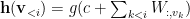
Each word 

The output layer requires a softmax function to compute the word probability. A hierarchy softmax is necessary to scale up this calculation.
DocNADE Language Model
The previous model may not suitable for language model because it focuses on learning a semantic representation of the document. The hidden layer now needs to pay more attention to the previous terms. It can be accomplished by using n-gram model:

The additional hidden unit $latex \textbf{h}_i^{LM}$ models a n-gram language model:
$latex \textbf{h}_i^{LM}(\text{v}_{<i}) = \sum_{k=1}^{n-1}U_k \dot W_{:,v_{i-k}}^{LM}$
The matrix 

Summary
DocNADE is similar to Recurrent Neural Network model where both models estimate the conditional probability of the current input given the previous input. For language modeling task, RNN is less explicit on how much word or context to look back. But DocNADE requires us to explicitly tell the model the number of words to look back. On the other hand, DocNADE has a similar favor to Word2Vec where the document representation is simply an aggregate of all previously seen words. However, DocNADE adds additional transformation on top of hidden units.
Will this type of Autoregressive model fall out of fashion due to the success of Recurrent Network with Attention mechanism and memory model? The current trend suggests that RNN is more flexible and extensible than NADE. Hence, there will be more development and extension of RNN models more and more in the coming year.
References:
Lauly, Stanislas, et al. “Document neural autoregressive distribution estimation.” arXiv preprint arXiv:1603.05962 (2016).
 or
or  which is different from the discriminative model which estimates a conditional probability
  directly. An autoregressive model is one of three popular approaches in deep generative models beside GANs and VAE. It models
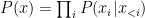
 where d is an index of the permutation o. For example, if we have
  , and o = {2, 3, 4, 1}, then
  . The permutation of the observation is more generic notations. Once we model the observation, the hidden variables can be computed as:
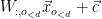
 And we can generate the observation ( a binary random variable) using a sigmoid function:
 recursively:

 can be done in a linear fashion.
You must be logged in to post a comment.