Day3-s: Lambda Learner

The main challenge in many machine learning models is to keep the model up-to-date with the latest dataset. The model refresh frequency could be within a day, an hour, or even a second. With the rapid change in users’ contents and behaviors over the web, the near real-time model training and refreshing are crucial for any organization to recommend relevant products to the key customers. But to achieve this goal has posed a few challenges. This paper proposes a solution to this matter.

Lambda Architecture

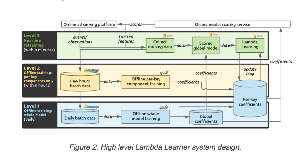
This paper is inspired by Lambda architecture. The batch data and real-time data pipeline are aggregated to keep the data as fresh as possible. Can we utilize this idea in the model training? For instance, the spam detector is currently trained on the past month’s datasets. Then the hackers suddenly change the algorithms. Then, the spam coming to the detector will have different characteristics and our detection may fail to catch the spam messages.

The model retraining approach can be classified into 4 levels:

• Stationary problem – train once and done
• code-start retraining – retrain the entire model periodically
• warm-start retraining – retrain a specific component of the model once there is enough data
• nearline retraining – asynchornously nearline on streaming data

Another takeaway is that the training must be lightweight for a near-real-time model refresh while stationary training can be done offline with a much larger accumulated dataset.

Data is collected by taking the features used by the model as soon as the model is used. Then, combine the features with the relevant engagement (click). In their use cases, the ads model scores the given ads. The feature will be saved. Then, as soon as the ad is clicked, the click data will instantaneously be combined with the saved features.

But to re-train the model, the mini-batch should not be too small. Otherwise, the learning will be unstable. Typically, for their application, the mini-batch has 100 examples that could be easily collected in seconds.

Finally, the near real-time model is not perfect. Although the model performs much better than the model trained offline when there is a change in the data, the model starts to accumulate more and more errors, which eventually degrade the model’s overall performance. The authors observed that the model can last for 60 hours without a full-batch update.

This is a great idea to have an infrastructure to main multiple models with different levels of data freshness. This is suitable for those applications that need to react to the surge of changes.

Reference:

• https://arxiv.org/pdf/2010.05154.pdf
• https://engineering.linkedin.com/blog/2021/lambda-learner–nearline-learning-on-data-streams

Day7-r: Multi-step Conversions with Multi-task Learning

In the e-commerce, the labels are usually impression, clicks, add to cart, and order. The ranking model is typically trained on these labeled data. It is possible to design multiple objective function using these labels.

One key observation is that these labels are strongly depended on one another. For instance, a merchandise item would not be purchased if it was never clicked. This work attempts to model these label relationship through the sequential models.

The model is trained to predict the clicks, impression, atc, etc. For each label, the hidden representation is created through the feed forward networks. Due to the sequential dependent between clicks, atc, impression. The hidden representation for clicks is a function of the impression; and same for ATC as well as the number of orders. The simple recurrent neural nets is used to learn these hidden representation.

The multi-objective functions are weighted by the learnable weight parameters. One modification to the objective function is to enforce the predicted impression to be greater the predicted clicks and so on.

In sum, for some instances of the multi-task learning problem, we can try to make each task to be correlated. This idea seems to be useful in the e-commerce application.

Reference:

• https://arxiv.org/pdf/2105.08489.pdf

Node2Vec: Scalable feature learning for networks (KDD’16)

Intro

This paper proposes a generalization of DeepWalk [2] and Line [3].

Key Ideas

The key observation is that the role of the vertex is also important. For example, given two vertices that are far apart from each other but share similar kind of vertices. Then, they both have similar roles (e.g. hubs or bridges). Breadth-First-Search traversal can capture this graph structure. On the other hands, the community is described as reachability/closeness of the two nodes in the graph. For instance, in the social network, my friend’s friend’s friend has a higher chance to belong to the same community as me.

Similar Works

DeepWalk uses a random walk to create a set of vertices that represents a context around the vertex of interest. The path generated by the random walk will either lead to the very faraway node or nodes around the seed. The context that is captured by this process can be unpredictable and depends on the graph structure.

Line focuses on neighbor vertices, which is the same as Breadth-First-Search traversal (BFS). In this case, it captures the local community in the graph.

Node2Vec

It comes down to what is a proper way to define the walk so that we can capture both community structure and role-based structure. Node2Vec defines a general method of graph traversal that is controlled by 2 parameters, p and q.

The key difference between BFS and DFS samplings is that the BFS is better at exploring the local neighborhoods while DFS is good at exploring larger parts of the network. BFS is viewed as micro-view of the graph whereas DFS characterizes the macro-view of the graph. The authors believe that the mixture of these two classic sampling will improve the representation of the graph embedding.

Search bias

The unnormalized transitional probability from node v to x is:

if

if

if

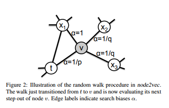
Where t is the previously visited node, v is the current node, and x is the next node. The distance determines the type of visiting nodes. When the distance between the previous node t and the next node x is zero, it means that we return to the node t.

However, when the distance is 1, it means that we want to visit the node that is directly connected to current node v and the previous node t. It means that node x is shared node between v and t. Hence, this walk will capture the structure of the network (local view).

Lastly, when the distance is 2, we want to hop further away from node t. This is similar to DFS where we want to go deeper into the network graph.

Parameter p and q will control the characteristic of bias walking. The high value of p means that we don’t want to go back often. The high value of q means that we do not want to make too many hops. Hence, p and q control the balance between BFS and DFS sampling.

Closing

This paper generalizes the random walk by adding parameters to control the walk characteristic. I think this is a neat idea because some information networks may need a specific walk than a general random walk. Thus, this model allows us to define the context based on how much we want to explore the network versus how much we want to exploit the local structure.

References:

[1] Grover, Aditya, and Jure Leskovec. “node2vec: Scalable feature learning for networks.” Proceedings of the 22nd ACM SIGKDD international conference on Knowledge discovery and data mining. ACM, 2016.

Click to access 1607.00653.pdf

[2] Perozzi, Bryan, Rami Al-Rfou, and Steven Skiena. “Deepwalk: Online learning of social representations.” Proceedings of the 20th ACM SIGKDD international conference on Knowledge discovery and data mining. ACM, 2014.

[3] Tang, Jian, et al. “Line: Large-scale information network embedding.” Proceedings of the 24th International Conference on World Wide Web. International World Wide Web Conferences Steering Committee, 2015.

DeepWalk: Online Learning of Social Representation (KDD’14)

DeepWalk is a novel approach for learning a latent representation of vertices in a network. The problem is summarized as we are given a graph containing edges and vertices, we want to embed each vertex into an embedding space.

How does DeepWalk work?

The idea behind this model is that vertices that are near each other should have similar latent vectors. So it really comes down to how to define a set of similar vertices. Interestingly, there is a connection between graph and natural language. The authors show that the distribution of words in natural language, as well as distribution of vertices appearing in short random walks, follow a power-law.

This means that a random walk starting at any random vertex is the same as modeling a symbol frequency. Hence, we can use a language model to estimate the likelihood of vertex appearing the given random walk.

Basically, DeepWalk model wants to learn a mapping function that will maximize the following likelihood function:

But the above likelihood function becomes more expensive to compute as the length of the walk grows. Hence, they use similar relaxations found in word2vec including word orderless, fixed window size, and skip-gram.

Now, the likelihood has changed to:

This model is the same the Skip-gram model in word2vec. The author uses a hierarchical softmax to model equation 1.

To train the model, the authors will go through each vertex in the graph, perform a random walk of length t, then optimize the objective function.

This is an interesting paper and shows the connection between graph structure and word embedding via the local context.

References:

[1] Perozzi, Bryan, Rami Al-Rfou, and Steven Skiena. “Deepwalk: Online learning of social representations.” Proceedings of the 20th ACM SIGKDD international conference on Knowledge discovery and data mining. ACM, 2014.

Click to access 1403.6652.pdf

FISM: Factored Item Similarity Models for Top-N Recommender Systems (KDD’13)

Sparsity is always the main problem in top-N recommendation models because we cannot observe all possible user and item interactions. This model aims to solve this problem by borrowing ideas from the two existing models: SLIM and NSVD models.

SLIM [1] model is a generalization of ItemKNN model. Instead of imposing a similar metrics such as Pearson correlation in order to identify similar items, SLIM learns a similar matrix from the data. Thus, the predicted rating of user u is:

This equation is simply a regression model. We want to predict a rating of item i by a user u by performing a linear combination of all rated items by a user u. The optimization problem of SLIM introduces a constraint term that forcing all diagonal of S to be 0. This prevents the model to do a self-predicted ( using a rating of item i to predict a rating of item i). It also added a nonnegative constraint so that the predicted rating is positive aggregations over items. It also has an L1 regularizer on S to force sparsity on S.

NSVD [2] model assumes that a similar matrix can be factored into two low-rank matrices.  The intuition behinds this is that two similar embedding item vector should yield a higher similarity score. The predicted rating of item i by user u is:

This equation states that a rating of item i by user u is an aggregation of all similarity score between item i and all items rated by user u (including an item i itself!)

FISM model simply extends NSVD model by making simple changes:

• It excluded item i from the NSVD formulation to avoid self-predicted rating.
• It added a normalization term to control the degree of agreement between the items rated by the user with an item whose rating is being estimated.

The FISM model is:

When the term is 1.0, the model will average all similarity scores. If all rated items have a high rating, then the predicted rating will likely to be high. On the other hand, when  term is 0.0, only few items with high rating can force the predicting rating to be high.

FISM paper proposed two learning model: FISMrmse and FISMauc. The first model is minimizing the square-loss between known rating and predicted rating. The second model is minimizing the rank-loss by placing a higher rated item before a lower rated item.

The experimental results show that FISMrmse is better than FISMauc based on Hit Rate and Average Reciprocal Hit Rank metrics. The NSVD is not part of the baselines since it solves rating prediction not top-N recommendation problem. In my opinion, FISM is not different from NSVD at all. FISMrmse is very similar to NSVD model except that it excludes item i.

References:

[1] X. Ning and G. Karypis. Slim: Sparse linear methods for top-n recommender systems. In ICDM 2011.

[2] A. Paterek. Improving regularized singular value decomposition for collaborative filtering. In Proceedings of KDD Cup and Workshop, volume 2007, pages 5-8, 2007.

[3] Kabbur, Santosh, Xia Ning, and George Karypis. “Fism: factored item similarity models for top-n recommender systems.” Proceedings of the 19th ACM SIGKDD international conference on Knowledge discovery and data mining. ACM, 2013.