Day4-r: Birch

One major limitation of monoBert is its inability to process a long document. monoBert truncates the concatenation of query and document tokens within 512 tokens. This could be a sub-optimal when we are dealing with a long document. There are many works recently propose a solution for applying Bert for a long document.

For this paper, the approach proposed for allowing Bert to process a long document is somewhat unexpected. The authors simply do not let Bert process a long document at all. Instead, they treat each sentence within the same document as an individual document. By doing this, they can avoid pass a long document to Bert model.

The first insight that the authors exploit is that only a few sentences in the documents are sufficient to represent the entire document (at least for a passage ranking task). This is somewhat surprising because we could end up losing a lot of information from the document. The way they compute the document score for the given query is to use the Bert to score all pair of (query, sentence), then pick the top 3 pairs with the highest scores, then the sum of these scores is the relevant score for this long document. This is a pretty simple idea and it works.

Another finding that the authors found has to do with the transferring. They found that Bert model is effective as transferring the knowledges from one domain to another. They found that by fine-tuning the Bert with Twitter ranking dataset, then fine-tuning one more time with the domain-specific task gives a significant boost in the performance. This demonstrates how well Bert can capture the common knowledge between two datasets.

Reference:

• https://www.aclweb.org/anthology/D19-3004.pdf

Day2-r: duoBert

From the paper from day 1, it shows that a simple Bert architecture can outperform the state-of-the-arts neural IR models on re-ranking task. The natural extension of the previous work is to change the loss function from point-wise loss to pair-wise loss. They called the pair-wise model as duoBert and the original point-wise model as monoBert. But this extension would’t be interesting enough.

Hence, the authors cascades the BM25 with monoBert and duoBert as a multi-stage ranking. This approach is well-known in the industry because duoBert is too slow to rank all documents. It is more latency-friendly to employ a lesser complex model to filter out uninteresting items so that duoBert will only focus on interesting items.

By cascading BM25, monoBert, and duoBert all together, the authors show that they can achieve the best recall. Here is the architecture:

Multi-stage ranking: BM25 -> monoBert -> duoBert

What I found from this paper that might be useful is the aggregation function. In the duoBert, the model computes the relevant score by comparing two input documents, p(d1, d2). In order to rank multiple documents, the model needs to compute the relevant scores for all possible pairs of documents. Specifically, the They tried different aggregation function and shows that summing and binary function work quite well.

Reference:

• https://arxiv.org/pdf/1910.14424.pdf

Day1-r: Passage Reranking with Bert

This is one of the early works that applies Bert architecture to the search problem. In search problem, there are two main stages: retrieval and re-ranking stages. The retrieval stage deals with retrieve relevant documents from a large candidate set. This stage must be fast and efficient but does not need to be accurate. The reranking stage is more concerned with rank the small set of documents. This stage allows the more computational expensive model such as Bert. This paper focuses on the re-ranking stage.

Bert has made a significantly impact to NLP and IR research communities. This paper proposes a simple search architecture for document re-ranking.

The architecture is as follows:

The model architecture proposed by this work

The authors fine-tune the Bert model on MS MACRO (400M tuples of a query, relevant and non-relevant passage) and TREC-CAR (2.3M queries) datasets using the cross-entropy loss as an objective function.

The results look promising:

This work demonstrates that even we apply the relevant/non-relevant passage data directly to the Bert model, the model has already outperformed many state-of-the-arts neural ranking models.

The main drawback could be that this model is only applicable for the reranking stage because it has to compute the relevant score for all documents which might be too slow when we are dealing with a large number of documents (1M+). Hence, the number of passages to rank can be limited for any practical search application.

Reference:

[1] https://arxiv.org/pdf/1901.04085.pdf

Day 0 : I am back.

I haven’t been writing blog posts for a few years since I have started my new job. For the past year, I have been actively writing blog/post at my company’s internal blogs and focusing more on the production and technical details related to my company’s roadmap.

However, it is also a time for me to get back to my public blogging and start to contribute what I have learned back to the community again.

I have been switching my focuses quite a bit. I hope to keep my 100 days learning going. I will start from the day 0.

I look forward for the fun ride.

Day 15: CVAE with Gumbel-softmax (cont)

My Day 14, I added Gumbel-softmax to sample a digit category but the result did not look good. I have found that switching from a straight-through Gumbel-softmax to a general Gumbel-softmax greatly helps the CVAE to learn a digit distribution.

Here are the results:

The result also looks much better than the generated digit by the method used in Day 13 (expanding the expectation term). It is partly because we do not average out the loss anymore.

I am surprised that a straight-through Gumbel-softmax does not quite work. Although I did use temperature annealing technique ( slowly convert a Gumbel-softmax to a straight-through Gumbel on the backward pass ), the result was not good.

It seems at this point, a general Gumbel-softmax performs much better, at least, for MNIST digit generation task.

 

Day 14: CVAE with Gumbel-Softmax

From my previous post, expanding the expectation term is not scalable when the dataset has many classes. For MNIST dataset with only 10 classes, the training is slow because we have to compute loss for all classes before applying a weight average.

For a gaussian distribution, we use reparameterization trick to convert a sampling step to a deterministic operation:

By using shift and scaling operations, we now have:

Where is an extra input to the network and we generate it from a Gaussian noise .

In our case, we also need another reparameterization trick for a categorical distribution. Gumbel-Softmax [1] is a surrogate function to approximate this sampling process. I will leave some technical details for my later post such as why choosing the Gumbel distribution is suitable and why softmax is used to approximate onehot vector representation.

For now, I simply added Gumbel-softmax into my CVAE. PyTorch provides a nice API for Gumbel-Softmax, so I don’t have to implement myself. Note that, there are two version of Gumbel-softmax: (1) Straight-through and (2) Non-Straight-through.

The Non-Straight-through Gumbel outputs a soft-version of a onehot encoder. It is possible that more than one entry has a non-zero value. The straight-through Gumbel (ST-Gumbel) simply outputs a one-hot encoder. However, during the backprop, ST-Gumbel uses a gradient from Non-ST gumbel.

Here are some initial results (without hyper-parameters tuning):

The output does not look correct. This could be the way I train the model because the original Gumbel-Softmax paper can train Semi-supervised VAE. This is something I will address next time.

References:

[1] https://arxiv.org/pdf/1611.01144.pdf

Day 13: Implementation of Semi-supervised VAE

This post is a continuation of my Day 12. To train semi-supervised VAE, we need to expand the expectation as follows:

The first term turns out to be the same loss as the standard CVAE. The second term is the entropy of the .

Entropy Loss

The entropy is an average information required to encode the given event. In our case, the event is the outcome of image prediction.

When entropy is high, it means we need to use more bits to encode the event. The highest entropy is when is a uniform distribution. This implies that if the discriminator cannot classify the images, the entropy will be high. When is no longer a uniform distribution, it hints us that the discriminator at least learns something. By minimizing the entropy, we encourage the model to learn some useful distribution instead of a boring uniform distribution.

Implementation (Pseudocode)

The implementation is as follows:

• for each mini-batch batch_x
  • for each class y
    • loss(x, y) = compute CVAE loss of batch_x and y
  • Avg loss = q(y|x) * loss(x, y)
• Avg loss += compute entropy loss for the current batch_x

This implementation can be slow during the training because we have to compute the loss for each class. If we have a lot of classes, it will be very slow.

Image generated by CVAE. We use 60 labeled images per classes.

Imaged generated by semi-supervised VAE. We use 60 labeled images and 5400 unlabeled images per class.

To be honest, the results are not impressive. The training could be better. Currently, I simply alternate between training labeled data and unlabeled data.

Next:

Another approach is to use an approximation of discrete output. One of the nice approximation is Gumbel-softmax which I will use and possibly implement it for my Day 14.

 

 

 

 

Day 12: Handling Discrete output in VAE

The limitation of GANs and VAE is that the generator of GANs or encoder of VAE must be differentiable. This prevents the model to generate a discrete output which can be useful for many tasks.

I start my study with Semi-supervised VAE [1].  This model is the same as CVAE but with an extra component for handling the unlabeled training dataset.

 

A semi-supervised model for VAE proposed by [1]

When the input has a label, we use the first architecture (which is CVAE) to train the model. When the input does not have a label, we use a discriminator to predict a label first. Then, we train the same way as labeled data.

To see the impact of unsupervised learning component, we can investigate the improvement of the generated images from the generator after adding unlabeled data.

First, we want to see how bad of the generated images after we train CVAE with the limited number of training samples:

Take 100% of images from each class (6000 images per class)

Take 10% of images from each class (600 images per class)

Take 1% of images from each class (60 images per class)

Take 0.1% of images from each class (6 images per class)

It is obvious that we don’t have enough data for VAE to approximate the image distribution.

Dealing with the Discrete output

It is quite straightforward to predict the label of the given unlabeled image first. But the real issue is that we cannot train CVAE end-to-end anymore because the output from the discriminator is a discrete output. We need to find the way to handle this situation.

Compute the Expectation directly (No Monte Carlo approximation)

The first approach to handle the discrete output from the encoder is to average out the reconstruction error for all possible discrete output. This is exactly what [1] did.

We factor and derive the ELBO:

Instead of sampling a label from , [1] side-steped by expanding the expectation term. This approach is workable for the dataset with the small number of classes but it is not scalable when we have a lot of classes.

Reference:

[1] https://arxiv.org/abs/1406.5298

Day 11: 2D one-hot representation

My last post, my CGAN’s architecture does not work and when it is trained, its generator will learn nothing (complete mode collapsing issue). After a few days of research and read a few tips online, I’ve found the architecture for CGAN that works!

Before I describe the specific architecture for CGAN, here are the results:

generated MNIST digits by CGAN. It is easy to interpret each row as a stroke width, stroke style.

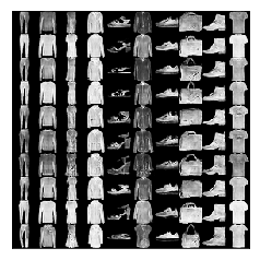
generated fashion items by CGAN. It is harder to interpret each row.

The loss of discriminator and generator look much better:

Loss on MNIST dataset

Loss on Fashion-MNIST dataset

The most important component of CGAN is the way we combine class label and actual image/latent vector as one input unit to the discriminator/generator. The choice of architecture either makes or breaks the model.

Generator

It takes two inputs: latent vector and class label.

• Latent vector is a random vector drawn from a normal distribution, mean at 0 with a unit variance.
• A class label is a one-hot vector.
• We concatenate these two vectors and use a few feedforward layers to merge them.
• Finally, we pass the new vector into deconvolutional layers.

Discriminator

It takes two inputs: generated image/real image and class label.

• Generated image or real image is a 2d matrix.
• a class label is converted to a 2d one-hot representation. This component was missing from my previous CGAN implementation. I will describe it a bit later.
• The generated/real image with 1 color channel + 10 channels from 2d one-hot representation.

2D one-hot representation

The idea is simple. For each class label, we represent it as 10 matrices ( or a matrix of size 10 by image width by image height ). For a class label i, the ith matrix is one matrix, the rest are zero.

This representation is simple and combines nicely with the actual 2d image. I will explore deeper into this choice of representations and how it might affect the discriminator.

References:

[1] https://arxiv.org/abs/1411.1784

 

Day 10: Mode Collapsing on my CGAN

I tried to implement a conditional GAN [1]. At first, it seems to be a straightforward extension of GANs. But I ran into a mode collapsing and it was a mess:

Here are digit 5 generated by the conditional GANs:

Epoch 10:

Start off, it looks okay.

Epoch 50:

wait, the model ignores the class label.

Epoch 100:

So the generator was giving up now?

Epoch 150:

Yup, it is a complete mode collapsing. The generator just gave up.

This is not good. I need to find the right architecture for CGAN or the appropriate hyperparameters.

Ideally, what I want to achieve should look like this:

This is not my image!

I expect to put more efforts in term of training the CGAN model and the pick the right choice of the architectures and hyper-parameters. Stay tune.

References:

[1] https://arxiv.org/abs/1411.1784