Day 6: DCGAN

After I spent a few days on an autoregressive model, I want to switch my focus on GANs for the coming days. Today I worked on DCGAN [1] which is GANs that uses a deconvolution network as a generator and a convolution network as a discriminator.

Although the use of deconvolutional layers may sound straightforward, I still like some ideas of DCGAN’s architectures:

1. It does not use any max-pool at all and uses a strided convolutional layers to down-sampling instead. The use of multiple convolutional layers for down-sampling was proposed by [2].
2. It uses a deconvolutional layer as part of the generator by slowly double the number of channels until it reaches the desired image dimensions.
3. This is a subtle idea. It uses LeakyReLU instead of ReLU.

I modified my Vanilla GAN by replacing the generator and discriminator with conv and deconv layers.

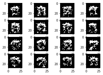
We randomly select 16 random vectors with a dimension of 64 drawn from a normal distribution. Each column represents one unique vector. Each row represents the number of epochs.

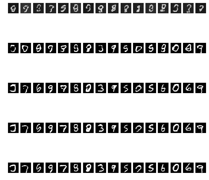
Sampled digits generated by the generator. Each row represents the number of epoch. From top to bottom: epoch 10, 50, 100, 150, and 200. We can see that the more epochs, the better image quality.

DCGAN generates much better image quality than Vanilla GAN. Hence, convolutional and deconvolutional layers give representation and classification power to the models.

Loss Plot

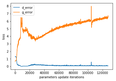
To be honest, the loss does not look good to me. I expected the loss from the generator slowly decays overtimes but that is not the case here. It seems that the discriminator performs a binary classification extremely well. This could be bad for the generator since it will never receive a positive signal, but only negative signals. The better training strategy will be explored in my future study.

Closing

DCGAN is a solid work because the generated images are significantly better than Vanilla GANs. This simple model architecture is more practical and will have a long-lasting impact than a sophisticated and complex model.

Code

References:

[1] DCGAN original paper

[2] Striving For Simplicity: The All Convolutional Net  (ICLR’15)

 

Day 5: MADE – Mask Autoencoder

The main problem with NADE is that it is extremely slow to train and sample. When training on a MNIST digit, we need to compute log probability one pixel sequentially. Same goes for sampling a MNIST digit.

MADE – Mask Autoencoder [1] proposes a clever solution to speed up an autoregressive model. The key insight is that an autoregressive model is a special case of an autoencoder. By removing a weight carefully, one can convert an autoencoder to an autoregressive model. The weight removal is done through mask operations.

I used the implementation from [2] and trained MADE with a single layer of 500 hidden units on a binary MNIST dataset. I sample each image by first generating a random binary image, feed it to the MADE, then sample the first pixel. Then, I update the first-pixel value of the random binary vector. I then pass this random vector to the MADE again and so on.

Here are sampled images:

They look pretty bad! I barely notice a digit 7. This makes me wondered if a single layer MADE is not strong enough or the way I sample an image is not correct.

The strength of MADE is that training is very fast. This contribution alone makes it possible to train a large autoregressive model. I really like this paper.

References:

[1] https://arxiv.org/pdf/1502.03509v2.pdf

[2] https://github.com/karpathy/pytorch-made