Before I dive into some advance autoregressive models, I want to step back and implement NADE model proposed by Hugo et al [1]. Last year I wrote a blog post about this model but never implement the model. Hence, I will dedicate my day 4 on implementing NADE model.
The autoregressive model is similar to RNN. It is a sequential model and assumes that the current input depends on the previous inputs.

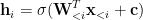
Then, the hidden state can be computed by a shared weight variable W:
Then, we compute the log-likelihood as follows:

NADE shares weight parameters so it only has one neural nets to transform the sequential data into a series of hidden variables.
However, training and sampling data from NADE are very slow. For training and sampling, we need to sequentially compute each hidden variable. This is extremely slow even for a small image such as MNIST (32×32). The recent work such as Mask Autoencoder [2] has addressed this slow training issue.
References:
[1] http://proceedings.mlr.press/v15/larochelle11a/larochelle11a.pdf
[2] https://arxiv.org/abs/1502.03509
